CUDA error: out of memory

If you’ve ever tried to train a deep learning model, the dreaded CUDA error: out of memory is likely all too familiar. The usual quick fix is to decrease the batch size and move on without giving it much thought. But have you ever wondered about how memory gets allocated during training?? In this blog post, I want to demystify memory consumption during model training and and offer practical methods to reduce the demands of memory-heavy models.

Understanding Memory Consumption in Deep Learning

Before diving into the solutions, it’s crucial to understand what consumes memory during training. The main sources of memory usage are:

Model Weights: The parameters of your neural network.
Gradients: Calculated during backpropagation.
Optimizer States: Additional variables maintained by optimizers like Adam.

Additionally, there’s something called Residual Memory (a term coined by the ZeRO paper), which includes:

Activations: Outputs from each layer needed for backpropagation.
Temporary Buffers: Used for intermediate computations.
Memory Fragmentation: Wasted memory due to how GPUs allocate memory blocks.

Let’s break these down.

The Adam Optimizer: A Quick Refresher

If you’re already familiar with the Adam optimizer, feel free to skip this section. If not, here’s a brief overview to ensure we’re all on the same page.

1. Gradient Descent (GD)

Gradient Descent is the foundational optimizer used to minimize a loss function by iteratively updating parameters in the direction of the steepest descent (negative gradient).

Update Rule: $$ \theta_{t+1} = \theta_t - \eta \cdot \nabla L(\theta_t) $$

$\theta_t$: Parameters at iteration $t$
$\eta$: Learning rate
$\nabla L(\theta_t)$: Gradient of the loss function with respect to $\theta_t$

Limitations:

Fixed Learning Rate: Choosing an appropriate learning rate can be challenging; too high may cause divergence, too low may slow down convergence.
No Adaptation: Doesn’t adapt the learning rate based on the geometry of the loss surface, potentially leading to inefficient updates.

2. Introducing Adam Optimizer

Adam (Adaptive Moment Estimation) combines the advantages of two other extensions of GD: Momentum and RMSProp. It computes adaptive learning rates for each parameter by maintaining estimates of both the first moment (mean) and the second moment (uncentered variance) of the gradients.

Key Concepts:

Momentum:
- Helps accelerate Gradient Descent in the relevant direction and dampens oscillations.
- Maintains an exponentially decaying average of past gradients.
RMSProp:
- Adaptive Learning Rates: Adjusts the learning rate for each parameter individually based on the magnitude of recent gradients.
- Parameters with higher gradients receive smaller updates, and vice versa.
- Moving Average of Squared Gradients: Maintains a moving average of squared gradients to normalize parameter updates, preventing vanishing or exploding gradients.

Adam effectively combines these by maintaining both moving averages (from Momentum and RMSProp) and adapting learning rates accordingly.

Adam’s Update Mechanism:

Adam maintains two estimates for each parameter $\theta$:

First Moment ($m_t$): Estimate of the mean of the gradients.
Second Moment ($v_t$): Estimate of the uncentered variance (mean of the squared gradients).

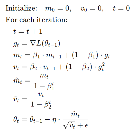
Update Steps:

Initialize Parameters:
- $m_0 = 0$ (first moment)
- $v_0 = 0$ (second moment)
- Choose hyperparameters:
  - Learning rate ($\eta$)
  - Decay rates for the moment estimates ($\beta_1$ for $m_t$, $\beta_2$ for $v_t$)
  - Small constant ($\epsilon$) to prevent division by zero
At each iteration $t$:
a. Compute Gradient: $$ g_t = \nabla L(\theta_{t-1}) $$
b. Update First Moment ($m_t$): $$ m_t = \beta_1 \cdot m_{t-1} + (1 - \beta_1) \cdot g_t $$
c. Update Second Moment ($v_t$): $$ v_t = \beta_2 \cdot v_{t-1} + (1 - \beta_2) \cdot g_t^2 $$
d. Bias Correction: $$ \hat{m}_t = \frac{m_t}{1 - \beta_1^t} $$ $$ \hat{v}_t = \frac{v_t}{1 - \beta_2^t} $$
e. Update Parameters: $$ \theta_t = \theta_{t-1} - \eta \cdot \frac{\hat{m}_t}{\sqrt{\hat{v}_t} + \epsilon} $$

Algorithm Summary:

Residual Memory Consumption

Now that we understand the primary components consuming memory—model weights, gradients, and optimizer states—let’s explore Residual Memory, which includes:

Activations:
- Outputs of each sub-component (e.g., self-attention, feed-forward networks) within each layer.
- For large models, activations can consume significant memory. For example, training a 1.5B parameter GPT-2 model with a sequence length of 1,000 tokens and a batch size of 32 can consume around 60 GB of memory solely for activations.
- Mitigation: Activation checkpointing (or recomputation) saves memory by storing only a subset of activations and recomputing others during the backward pass. This can reduce memory consumption (e.g., from 60 GB to 8 GB) but introduces a computational overhead of about 33%.

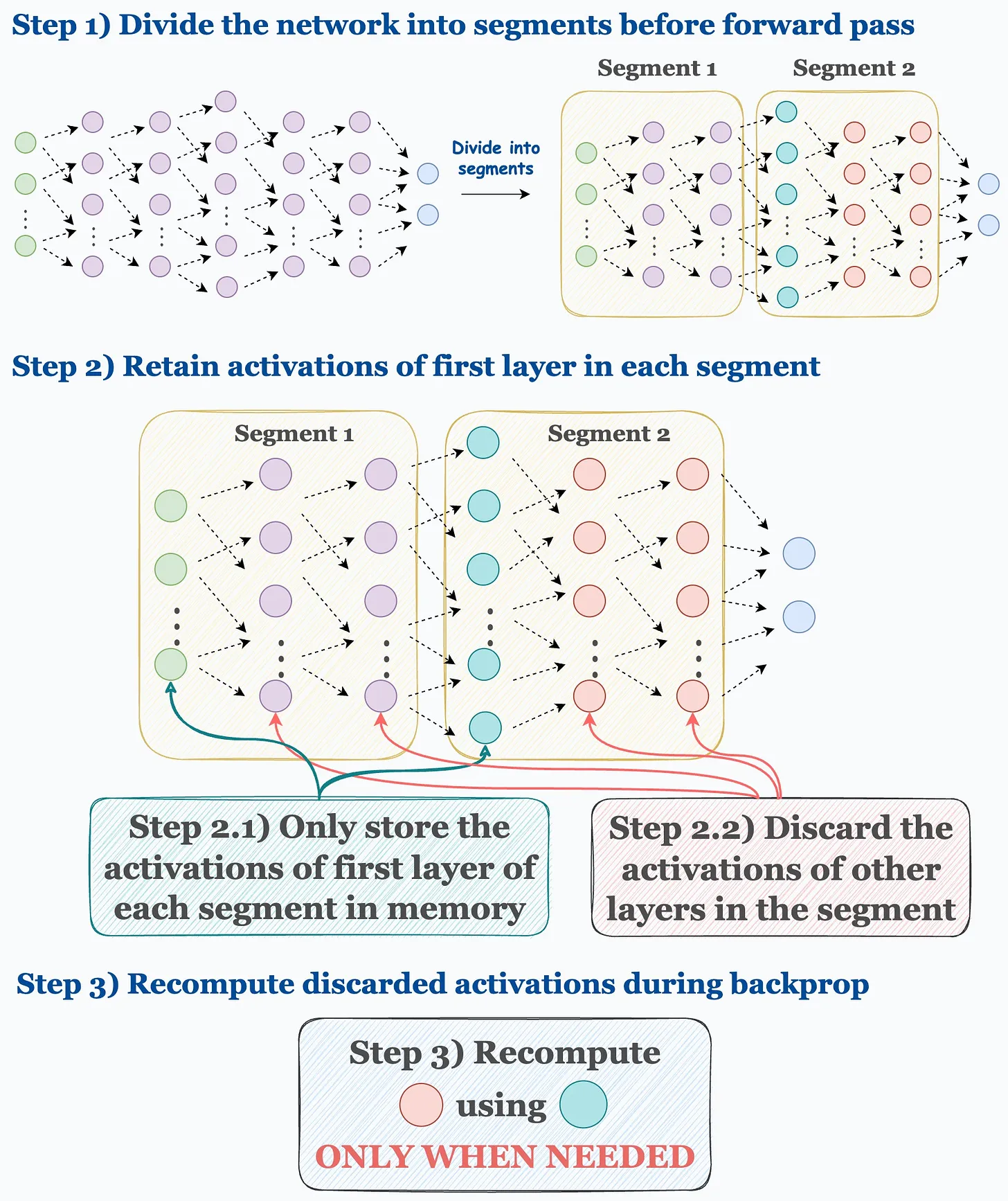
Figure 1: Activation Checkpointing Process. Source: Daily Dose of Data Science

Temporary Buffers:
- Store intermediate results during operations like gradient all-reduce (used in distributed training) and gradient norm computation (used for gradient clipping).
- For large models, temporary buffers can require significant memory. For instance, a 1.5B parameter model might need around 6 GB for a flattened FP32 buffer used during gradient all-reduce operations.
Memory Fragmentation:
- Even with considerable available memory, fragmentation can cause Out-of-Memory (OOM) errors because the GPU allocates memory in blocks. If there’s space for some parameters but not enough contiguous space for all, OOM errors occur.
- Example: Training extremely large models might fail with over 30% of memory still free but unusable due to fragmentation.

Figure 2: Memory Fragmentation in GPU Training. Source: Daily Dose of Data Science

Unfortunately, Residual Memory consumption is largely out of our control. However, understanding where the memory goes is essential for optimizing what we can manage.

Controlling Memory Consumption: Model Weights, Gradients, and Optimizer States

Now, let’s focus on the memory components we can control: model weights, gradients, and optimizer states.

Mixed Precision Training: A Memory-Saving Technique

While you can store all components in FP32, it’s often unnecessary. Mixed Precision Training is a widely adopted technique in the industry that involves storing some components in lower precision (e.g., FP16) to save memory.

How Mixed Precision Training Works

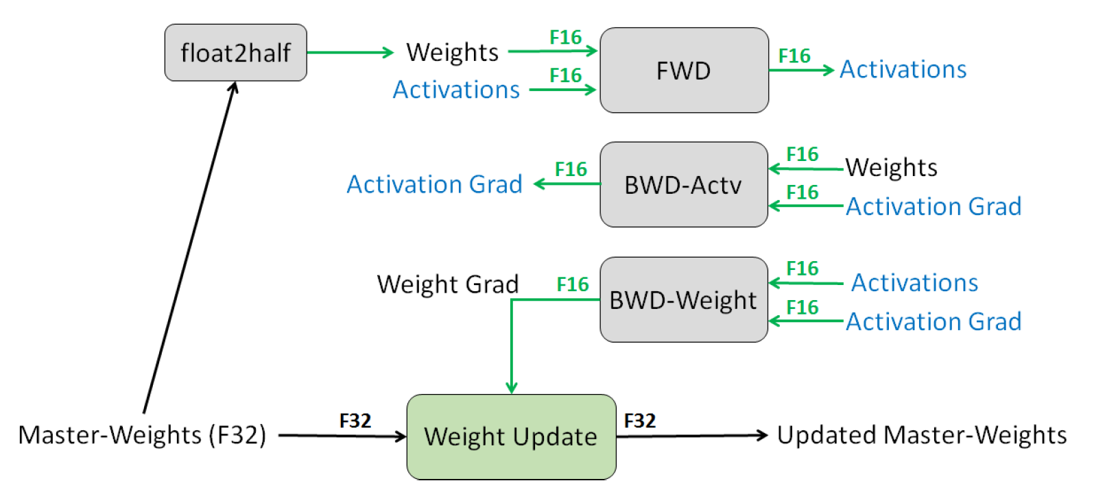
Figure 3: Mixed precision training iteration for a layer. Source: Narang et al. (2018)

Mixed Precision Training leverages both FP16 and FP32 data types:

Parameters and Activations: Stored as FP16, enabling the use of high-throughput tensor cores on NVIDIA GPUs.
Optimizer States: Maintained in FP32 to ensure numerical stability during updates.

During mixed-precision training, both the forward and backward propagation are performed using FP16 weights and activations. However, to effectively compute and apply the updates at the end of the backward propagation, the mixed-precision optimizer keeps an FP32 copy of the parameters as well as an FP32 copy of all the other optimizer states.

Memory Computation

Mixed precision training for a model with $ \Psi $ parameters, an FP16 (16-bit floating point) copy of the parameters requires $ 2\Psi $ bytes of memory. During training, gradients of these parameters are also computed and stored in FP16 format, which consumes another $ 2\Psi $ bytes.

In addition to the parameters and gradients, Adam maintains optimizer states to efficiently update the model during training. These optimizer states include an FP32 (32-bit floating point) copy of the parameters, as well as momentum (first moment estimates) and variance (second moment estimates) for each parameter. Each of these three components—parameter copies, momentum, and variance—requires $ 4\Psi $ bytes of memory, totaling $ 12\Psi $ bytes for all optimizer states.

Combining these components, the total memory requirement for mixed-precision Adam training becomes: $$ 2\Psi \ (\text{FP16 Parameters}) + 2\Psi \ (\text{FP16 Gradients}) + 12\Psi \ (\text{FP32 Optimizer States}) = 16\Psi \ \text{bytes} $$

For example, consider the GPT-2 model, which has 1.5 billion parameters ($ \Psi = 1.5 \times 10^9 $). Plugging this into the equation: $$ 16\Psi = 16 \times 1.5 \times 10^9 \ \text{bytes} = 24 \ \text{GB} $$ This means that training GPT-2 with mixed-precision Adam requires at least 24 GB of memory. In contrast, storing only the FP16 parameters of the model would require just $ 1.5 \times 10^9 \times 2 $ bytes, which equals 3 GB. This comparison clearly illustrates that while mixed-precision training with Adam offers computational advantages, it significantly increases the memory usage—from 3 GB for the parameters alone to 24 GB when including gradients and optimizer states.

However, the FP16-FP32 precision scheme comes with its own set of challenges. Due to the restricted numerical range of FP16, this scheme can cause instabilities when training large models. Below is an excerpt from the BLOOM model training team, who shared their experiences in a blog post on Hugging Face:

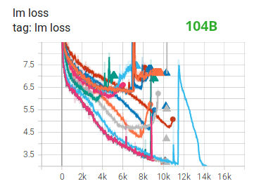
BF16Optimizer
Training huge LLM models in FP16 is a no-no. We have proved it to ourselves by spending several months training a 104B model which, as you can tell from the TensorBoard, was a complete failure. We learned a lot of things while fighting the ever-diverging LM loss:
We also received the same advice from the Megatron-LM and DeepSpeed teams after training a 530B model. The recent release of OPT-175B also reported significant difficulties in training with FP16.

This does not mean that you can’t train deep learning models using the FP16-FP32 precision scheme. However, for massive models with hundreds of billions of parameters, this approach is not the most effective.

Embracing BF16-FP32 Precision

So, should we abandon the hope for mixed precision training for massive llms? Absolutely not! You might remember from the quantization blog post my praise of the BF16 datatype. If you have a GPU with the Ampere architecture or later, you can leverage the BF16-FP32 precision format for mixed precision training. This approach is not fundamentally different from the FP16-FP32 scheme but offers significant advantages, especially for training massive language models.

Implementing Mixed Precision with BF16

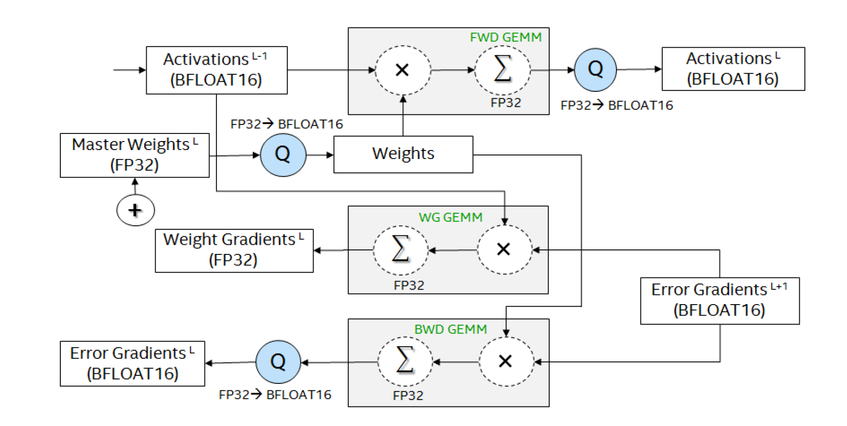
Figure 4: shows the mixed precision data flow used to train deep neural networks using BFLOAT16 numeric format. The core compute kernels represented as GEMM operations accept inputs as BFLOAT16 tensors and accumulate the output to FP32 tensors. Source: Kalamkar et al. (2019)

Here’s a more concise explanation of the mixed precision data flow using BFLOAT16:

Input: Activations from the previous layer (L-1) in BFLOAT16.
Forward Pass:
- Multiply BFLOAT16 activations with BFLOAT16 weights.
- Accumulate results in FP32.
- Quantize output to BFLOAT16 for the next layer’s input.
Backward Pass:
a. Error Gradients:
- Multiply BFLOAT16 error gradients with transposed weights.
- Accumulate in FP32, then quantize to BFLOAT16.
b. Weight Gradients:
- Multiply error gradients with transposed activations.
- Accumulate results in FP32.
Weight Update:
- Add FP32 weight gradients to FP32 master weights.
Precision Management:
- Store master weights in FP32.
- Use BFLOAT16 for computations and storage where possible.
- Perform critical accumulations in FP32.
- Convert between FP32 and BFLOAT16 as needed (shown as ‘Q’ operations).

This approach balances computational efficiency (using BFLOAT16) with numerical stability (using FP32 for critical operations), enabling effective training of large neural networks.

Since the BF16 datatype shares the same mantissa as FP32 (allowing it to represent the same range of values), you might wonder: Why not use BF16 for the optimizer states as well?

As you might correctly guess, training models in lower precision allows us to save memory and avoid numerical instabilities. However, an important question remains: Will models trained in lower precision be as effective as their FP32 counterparts if all other factors remain the same? To explore this issue, let’s examine the paper “Scaling Language Models: Methods, Analysis & Insights from Training Gopher” by Google DeepMind.

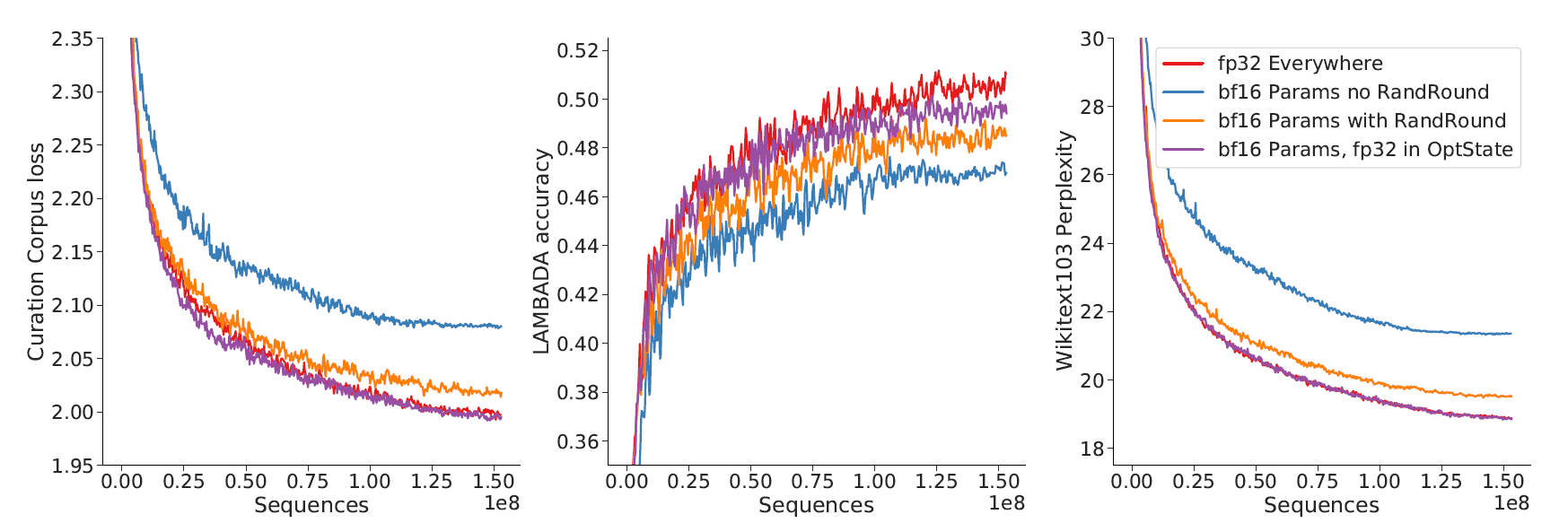
Figure 5: For four different combinations of float32 and bfloat16 parameters (detailed below) show performance on three different downstream tasks using a 417M parameter model. Source: Rae et al. (2021)

In this paper, the authors examined the effects of using the bfloat16 (bf16) numerical format compared to full float32 (fp32) precision for training large language models. They discovered that the optimal approach is to maintain float32 parameters solely for optimizer updates by storing a float32 copy in the optimizer state, while using bf16 for both model parameters and activations. This configuration effectively matches the performance of full fp32 training. The study tested four different precision configurations on a 417M parameter model across three downstream tasks, demonstrating that using a float32 optimizer state preserves key performance metrics—loss, accuracy, and perplexity—while leveraging the efficiency benefits of bf16 training.

Exploring FP8: The Next Frontier

The latest NVIDIA Hopper architecture and beyond support the FP8 format. Researchers have been exploring using FP8 to further optimize model training. However, instead of using FP8 as a data storage format, it is primarily utilized for GEMM (General Matrix-Matrix Multiplication) computations. The NVIDIA Transformer Engine (TE) applies FP8 solely for GEMM operations while retaining master weights and gradients in higher precision formats like FP16 or FP32.

Despite not offering substantial memory savings—since model weights are still stored in higher precision—FP8 calculations are twice as fast as FP16/BF16 computations.

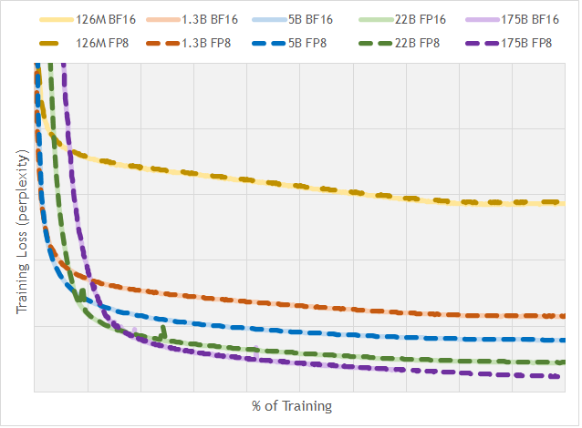
Figure 6: Training loss comparison across different floating-point formats and model sizes. Source: nai milra (FP8 FORMATS FOR DEEP LEARNING)

The results are quite impressive: FP8 achieves comparable performance to BF16, even for models scaling up to 175 billion parameters. This suggests that FP8 is a highly promising format for accelerating training without significantly affecting model accuracy.

Summary and Final Thoughts

Effective GPU memory management is a critical component in training large and complex deep learning models. Encountering the CUDA out-of-memory error is a common hurdle, but with the right strategies, you can overcome these challenges and optimize your training processes.

Key Strategies We’ve Explored:

Optimizer States: Understanding how optimizers like Adam maintain additional states helps in making informed choices about memory usage. Selecting memory-efficient optimizers or tweaking their configurations can lead to significant savings.
Mixed Precision Training: Utilizing lower precision formats such as FP16, BF16, and the emerging FP8 offers substantial reductions in memory consumption. These precision formats strike a balance between efficiency and maintaining model performance, making them invaluable for training large-scale models.

By implementing these strategies, you can train larger models more efficiently and avoid the common pitfalls of running out of GPU memory. Happy training!