Introduction to Quantization
Whether you’re an AI enthusiast looking to run large language models (LLMs) on your personal device, a startup aiming to serve state-of-the-art models efficiently, or a researcher fine-tuning models for specific tasks, quantization is a key technique to understand.
Quantization can be broadly categorized into two main approaches:
- Quantization Aware Training (QAT): This involves training the model with reduced precision, allowing it to adjust during the training process to perform well under quantized conditions.
- Post Training Quantization (PTQ): Applied after a model has already been trained, PTQ reduces model size and inference cost without needing to retrain, making it especially useful for deploying models efficiently.
In this post (and subsequent ones on this topic), we’ll focus on PTQ. It’s often a simpler starting point for quantization, providing a good balance between performance and implementation complexity. PTQ is particularly useful for deploying models to edge devices or serving them at lower hardware costs.
Why Quantization?
The costs of training large language models (LLMs) are already high, but inference costs—running the model to generate responses—can far exceed training costs, especially when deploying at scale. For instance, inference costs for models like ChatGPT can surpass training costs within just a week. Quantization helps reduce these costs by enabling models to operate in lower precision, such as FP16 or even INT4, without significant performance loss.
Let’s look at an example: suppose you want to run the LLaMA 3.1 8B model. What kind of memory and GPU would you need? If you load the model from Hugging Face, it will automatically be loaded in full precision (FP32). So, just to load the model weights, you would need:
$$ 8 \times 10^9 \text{ parameters} \times 4 \text{ bytes per parameter} \div 1024^3 \text{ for GB } \approx 30 \text{ GB} $$
This means you would need at least an A100 GPU with 40 GB of VRAM to load just the model weights. For fine-tuning, you would require around 90 GB, or a cluster of GPUs, and about 60 GB for inference.
This is where quantization can help. By loading the model in 8-bit, 4-bit, or even 2-bit precision, you can reduce your memory requirements by a factor of up to 16. If you load the same model in NF4 format (4 bits per parameter), you would need just around 5 GB to load the model, and about 12 GB for fine-tuning, which can be done even on a free-tier T4 GPU on Google Colab.
Understanding Precision in LLMs
If you’re unfamiliar with terms like FP32 or 8-bit precision mentioned earlier, don’t worry—we’ll cover them in the next section.
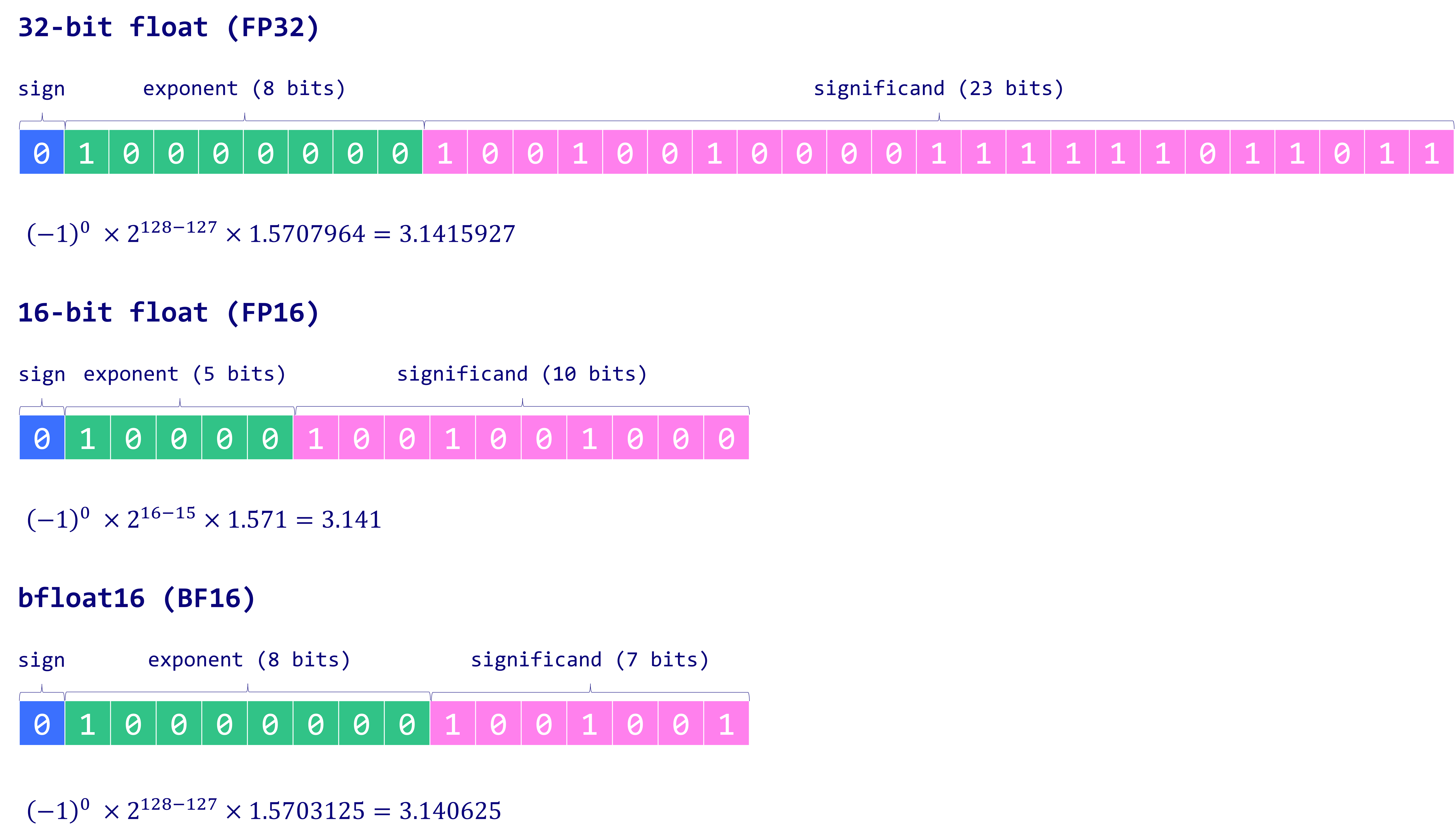
Comparison of 32-bit, 16-bit, and bfloat16 floating-point formats. (Maxime Labonne)
Starting with FP32
FP32 (32-bit floating point) is the most common datatype used to train deep learning models. If you don’t specify the datatype of tensors in PyTorch, FP32 is the default.
To understand how FP32 works and why it’s often preferred, let’s consider a simple example: representing the value of $\pi$ (pi) to 10 decimal places.
Precision in Deep Learning Models
Let’s assume we want to represent $\pi$ with the first 10 decimal places:
$$ \pi \approx 3.1415926535 $$
While this example is simple, it illustrates the inner workings of different data types like BF16 and FP16 — and later, we’ll discuss FP8, supported by the latest NVIDIA H100 GPUs and similar hardware.
How to Convert a Decimal Representation to FP32
To convert the decimal value of $\pi$ (3.1415926535) into its FP32 (single-precision floating-point) representation, follow these steps:
1. Understand the FP32 Structure
FP32 is composed of 32 bits, divided into three parts:
- Sign bit (1 bit): Indicates whether the number is positive or negative.
- Exponent (8 bits): Encodes the exponent using a biased format.
- Mantissa (23 bits): Represents the significant digits of the number.
2. Convert $\pi$ to Binary
We start by converting the decimal value of $\pi$ into its binary equivalent.
Convert the Integer Part:
The integer part of $\pi$ is 3. In binary:
$$ 3_{10} = 11_{2} $$
Convert the Fractional Part:
To convert the fractional part (0.1415926535) to binary:
- Multiply by 2 and record the integer part repeatedly:
- $0.1415926535 \times 2 = 0.283185307 \rightarrow 0$
- $0.283185307 \times 2 = 0.566370614 \rightarrow 0$
- $0.566370614 \times 2 = 1.132741228 \rightarrow 1$
- $0.132741228 \times 2 = 0.265482456 \rightarrow 0$
- $0.265482456 \times 2 = 0.530964912 \rightarrow 0$
- Continue this process to generate more bits.
The binary representation of $\pi$, up to a reasonable precision, is approximately:
$$ \pi \approx 11.001001000011111101101010100010_{2} $$
3. Normalize the Binary Representation
To fit the FP32 format, we need to normalize the binary number. Normalization involves adjusting the binary number so that there is only one non-zero digit to the left of the decimal point. We normalize this by shifting the decimal point one place to the left:
$$ 11.001001000011111101101010100010_{2} = 1.1001001000011111101101010100010_{2} \times 2^1 $$
This normalized representation is crucial for FP32 because the leading 1 before the decimal point is implicit and not stored, allowing the mantissa(the part after the decimal) to capture more significant digits. The exponent ($2^1$) indicates the scale of the number, while the mantissa captures the precise value.
4. Determine the Sign Bit
Since $\pi$ is positive, the sign bit is:
$$ \text{Sign bit} = 0 $$
5. Calculate the Exponent
In FP32, the exponent is stored using a biased representation. Bias is a fixed value added to the actual exponent to allow the encoding of both positive and negative exponents without using separate sign bit. For FP32, the bias is 127.
Calculating the Biased Exponent for $\pi$:
From the normalized form:
$$ \pi = 1.1001001000011111101101010100010_{2} \times 2^1 $$
- Actual Exponent: $1$
- Biased Exponent: $1 + 127 = 128$
Convert the biased exponent to binary:
$$ 128_{10} = 10000000_{2} $$
Thus, the exponent field in FP32 for $\pi$ is:
$$ \text{Exponent} = 10000000_{2} $$
6. Determine the Mantissa
The mantissa consists of the significant digits after the leading 1:
$$ \text{Mantissa} = 10010010000111111011010_{2} $$
Only the first 23 bits are kept; the rest are truncated, resulting in a small loss of precision. FP32 typically provides about 7 to 8 decimal places of precision. If more precision is needed, FP64 (double-precision) could be used, but for deep learning, FP32 is often more than sufficient.
7. Combine the Components
Now, combine the sign bit, exponent, and mantissa to form the final FP32 representation:
- Sign bit: 0
- Exponent: 10000000
- Mantissa: 10010010000111111011010
Thus, the FP32 representation of $\pi$ is:
$$ \text{FP32} = 0\ 10000000\ 10010010000111111011010_{2} $$
This is the IEEE 754 standard representation of $\pi$ in FP32 format.
FP16
The FP16 format uses fewer exponent and mantissa bits compared to FP32, This reduction results in a smaller range of values that can be represented. Specifically, in FP32, the largest representable number is approximately $3.4 \times 10^{38}$, while the smallest positive normal number is $1.175 \times 10^{-38}$
In contrast, FP16 reduces these limits: the largest representable number is approximately $6.55 \times 10^{4}$, while the smallest positive normal number is $6.10352 \times 10^{-5}$.
This reduction in range makes FP16 more limited when storing very large or very small values, which can affect the stability of models when when using FP16 for training.
Implications for Model Training and Fine-Tuning:
Loading FP32 Models in FP16: Simply converting an FP32 model to FP16 to fit it onto a GPU can lead to issues. The reduced range means that large weights or activations from the FP32 model might exceed FP16’s maximum representable value, causing overflow and resulting in “NaN” (Not a Number) errors during training.
Practical Solutions:
- Mixed Precision Training: A common approach is to use FP16 for most computations while keeping certain critical variables, like weights or gradients, in FP32. This balances the memory and speed benefits of FP16 with the numerical stability of FP32.
- Gradient Clipping: Implementing techniques like gradient clipping can help prevent gradients from becoming too large, mitigating the risk of overflow in FP16.
BF16
BF16, also known as Brain Float 16, was developed by Google Brain and became popular around 2019. It’s now one of the most widely used formats for training and fine-tuning LLMs. The main advantage of BF16 is that it retains the same number of exponent bits as FP32, making it easier to load a model in 16-bit precision and proceed with fine-tuning without running into “NaN” errors.
While BF16 sacrifices some precision compared to FP32, research has shown that the difference in performance when training or fine-tuning models on BF16 vs FP32 is minimal across different domains. Given the tradeoff between slightly reduced precision and the substantial reduction in model size, using BF16 is often well worth it for modern deep learning tasks.
More Data Types
TF32 (TensorFloat 32)
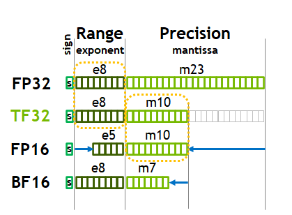
Comparison of floating-point formats: FP32, TF32, FP16, and BF16 in terms of range and precision. (NVIDIA A100 Tensor Core GPU Architecture)
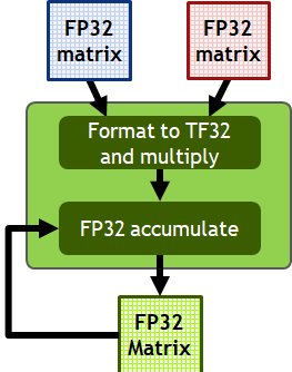
Matrix multiplication using TF32 format with FP32 accumulation. (NVIDIA A100 Tensor Core GPU Architecture)
TF32, or TensorFloat 32, is a special datatype introduced by Nvidia with the Ampere architecture (e.g., RTX 30 and A100 series) in 2020. Unlike FP16, which you can explicitly declare in PyTorch, TF32 is not directly accessible as a datatype in the framework. Instead, it is a precision format used specifically by the CUDA cores of the GPU for certain operations, particularly matrix multiplications.
From the Ampere architecture onwards, all calculations involving FP32 matrices are done as shown in the figure. When performing matrix multiplications, the GPU automatically converts FP32 matrices into TF32 precision. The actual multiplication is done using TF32, which retains FP32’s 8-bit exponent but reduces the mantissa to 10 bits. Once the operation is complete, the results are accumulated back into FP32 format for higher precision in the final outcome.
This process leverages TF32 for speed during calculations, while maintaining the precision of FP32 for the final result.
FP8 (E4M3 and E5M2 Formats)
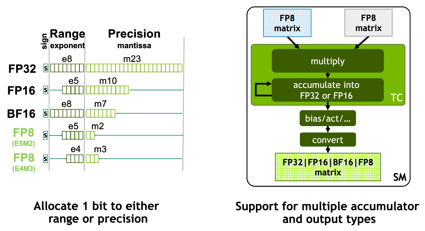
FP8 formats allocate bits between range and precision for efficient matrix computations. (NVIDIA H100 Tensor Core GPU Architecture)
FP8 is an emerging precision format designed to accelerate deep learning training and inference beyond the 16-bit formats commonly used today. Introduced in recent research paper FP8 Formats for Deep Learning from September 2022, FP8 comes with two encoding options: E4M3 (4-bit exponent, 3-bit mantissa) and E5M2 (5-bit exponent, 2-bit mantissa). FP8 was introduced as part of Nvidia’s Hopper Architecture (H100 GPUs).
The main advantage of FP8 is its ability to drastically reduce memory and compute requirements while maintaining comparable performance to higher precision formats like FP16 and BF16. The flexibility between the E4M3 and E5M2 formats allows FP8 to allocate an additional bit either to range or precision, depending on the task requirements.
As shown in the figures:
- FP8 calculations: Input matrices are converted to FP8, multiplied, and then accumulated in a higher precision format (FP16 or FP32). This allows for efficient computation while retaining enough precision in the final result.
- Efficacy of FP8: The graph below illustrates the training loss (perplexity) across various large models (GPT-3 variants with up to 175 billion parameters), showing that FP8 training closely matches the results achieved with BF16.
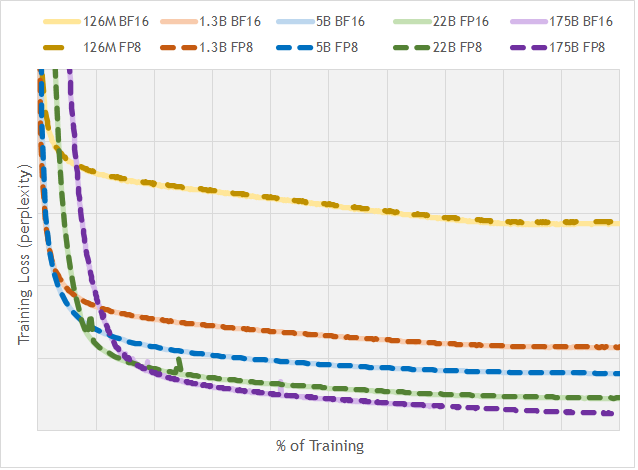
Training loss comparison across different floating-point formats and model sizes. Source: nai milra (FP8 FORMATS FOR DEEP LEARNING)
Nvidia is Everywhere!
Let’s address an important consideration. So far, I’ve mentioned that the TF32 datatype was introduced with Nvidia’s Ampere architecture and that FP8 support starts with the H100 GPUs. While we’ve been exploring these different data types, here’s something to keep in mind: you might be interested in using BF16 after reading this post, but if you try it on a free Colab instance with T4 GPUs, you’ll find that BF16 isn’t supported.
I’ve reviewed Nvidia’s whitepapers to save you the effort. It’s crucial to know the hardware you’re using and the data types it supports. This knowledge helps you choose the right GPU cluster for your projects.
Take a look at the chart below. The numbers represent FLOPs (or TOPs for INT data types), and the X’s indicate that a data type isn’t supported by a particular architecture. I’ll follow up with some key observations to help you navigate these choices effectively.
| GPU | P100 | V100 | T4 | A100 | H100 | L40 | B100 |
|---|---|---|---|---|---|---|---|
| VRAM | 16GB | 32GB | 16GB | 40GB* | 80GB | 48GB | 192GB |
| Architecture | Pascal | Volta | Turing | Ampere | Hopper | Ada Lovelace | Blackwell |
| Release Date | Apr-16 | May-17 | Sep-18 | May-20 | Mar-22 | Sep-22 | Mar-24 |
| FP32 | 10.6 | 8.2 | 8.1 | 19.5 | 67 | 90.5 | 60 |
| TF32 | X | X | X | 312 | 989 | 181 | 1800 |
| FP16 | 130 | 65 | 624 | 1979 | 362 | 3500 | |
| BF16 | X | X | X | 624 | 1979 | 362 | 3500 |
| INT8 | X | X | 130 | 1248 | 3958 | 724 | 7000 |
| INT4 | X | X | 260 | 2496 | 1448 | ||
| FP8 | X | X | X | X | 3958 | 724 | 7000 |
| FP4 | X | X | X | X | X | X | 14000 |
Some Observations
- Blank entries indicate supported data types for which I couldn’t find the exact values.
- Values highlighted in blue represent sparse matrices.
- INT4 and INT8 data types were introduced with the Turing architecture for inference.
Integer Qunatization
As you have already seen the T4 and Subsequnet gpu archtecture suppor INT8 and INT4 datatypes, thes datatypes can be used for inferecne and can be blazingly fast, (Just to keep another thing on the back of you mind is that if you load you matrix in a particula data type like INT8, this dosent necessarily mena the compuatations are Happening in IN8, will expand on this later)
ABS Max Quantization
Absmax quantization is a method used to convert floating-point values (like FP16) into 8-bit integer values. Here’s how it works in simpler terms:
Scaling factor calculation: The input tensor (a matrix of floating-point numbers, $X_{f16}$) is scaled based on its largest absolute value. To do this, the method computes the maximum absolute value of all the elements in the tensor, also called the infinity norm ($|X_{f16}|_\infty$). The scaling factor, $s_{xf16}$, is then calculated as: $$ s_{xf16} = \frac{127}{|X_{f16}|_\infty} $$ The value 127 is used because the 8-bit integer range is between $-127$ and $127$.
Quantization: Once the scaling factor is computed, the input tensor values are multiplied by $s_{xf16}$ to map them into the 8-bit range: $$ X_{i8} = \text{round}\left(127 \cdot \frac{X_{f16}}{|X_{f16}|_\infty}\right) $$ This means each value in the tensor is scaled down proportionally to fit into the [-127, 127] range, and then rounded to the nearest integer to make it an 8-bit value.
Effect: This process allows a tensor originally in a high precision format (FP16) to be represented using 8-bit integers, reducing memory usage and potentially speeding up computations at the cost of some precision.
In summary, absmax quantization shrinks a floating-point tensor into the 8-bit range by dividing all elements by the largest absolute value in the tensor, then multiplying by 127 and rounding.
LLM int8
Abs Max Quantization works, so shouldn’t we just wrap up quantization and move on? Not quite. In November 2022, Detmers et al. introduced LLM.int8(), a new quantization technique, addressing an important issue: Large language models (LLMs) have started to show impressive emergent behaviors like reasoning, in-context learning, and even few-shot problem solving—abilities that were being compromised by naive quantization methods.
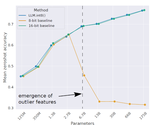
Accuracy trends with LLM.int8() showing the impact of outlier features as model size grows. (LLM.int8(): 8-bit Matrix Multiplication for Transformers at Scale)
The figure points out that once models exceed 2.7 billion parameters, naive 8-bit quantization significantly degrades performance. The drastic performance drop is due to the presence of outliers—weights that are crucial for enabling key behaviors like reasoning and in-context learning. These outliers are vital for the model’s performance, so preserving them during quantization is essential to prevent significant degradation. This happens because outlier weights—which play a crucial role in driving the emergent behaviors of large models—get lost in the quantization process.
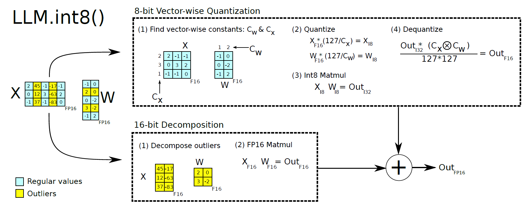
LLM.int8() proposes a two-part strategy to address this issue:
Vector-wise Quantization: Instead of quantizing the entire tensor with a single scaling constant, LLM.int8() quantizes vectors individually. The challenge with using a single scaling constant per tensor is that just one outlier can distort the entire quantization process, reducing precision for all other values. By applying multiple scaling constants—one for each vector—this method ensures that outliers don’t interfere with the rest of the matrix.
Mixed-Precision Decomposition: LLM.int8() quantizes only weights within a defined threshold, typically $[-6, 6]$. Outliers exceeding this range are preserved in higher precision formats (FP16 or FP32). This preserves critical outlier weights—crucial for model performance—at higher precision, avoiding accuracy loss from forcing them into lower precision formats. The approach maintains key model behaviors while achieving significant compression for most weights, effectively balancing performance and efficiency across varying model sizes.
Comparison of zero-shot accuracy for various quantization methods as model parameters scale. (LLM.int8(): 8-bit Matrix Multiplication for Transformers at Scale)
the Mathematical details
Vector-wise Quantization
In vector-wise quantization, the main idea is to apply different scaling constants for each vector in the matrix multiplication to reduce the impact of outliers on quantization precision.
Matrix Setup:
- Let $ X_{f16} \in \mathbb{R}^{b \times h} $ be the input matrix (e.g., hidden states), where $ b $ is the batch size and $ h $ is the hidden size.
- Let $ W_{f16} \in \mathbb{R}^{h \times o} $ be the weight matrix, where $ o $ is the output size.
The goal is to quantize these matrices from FP16 to Int8, applying different scaling constants to different rows or columns.
Quantization(similar to ABSMAX Quantization):
- Quantization scales the values in each vector of $ X_{f16} $ and $ W_{f16} $ into the range $[-127, 127]$. The scaling constant for each row in $ X_{f16} $ is denoted $ c_{x_{f16}} $, and for each column in $ W_{f16} $, it is $ c_{w_{f16}} $.
This can be represented as: $$ Q(X_{f16}) = \frac{127}{|X_{f16}|_{\infty}} X_{f16} $$ where $ |X_{f16}|_{\infty} $ is the infinity norm (the maximum absolute value of the vector).
Matrix Multiplication: The quantized matrix multiplication is then performed in Int8 precision: $$ C_{i32} = Q(X_{f16}) \cdot Q(W_{f16}) $$ Here, $ C_{i32} $ represents the result of the Int8 matrix multiplication.
Denormalization: To recover the correct FP16 result after quantization, the matrix result must be denormalized by the outer product of the scaling constants: $$ C_{f16} \approx \frac{1}{c_{x_{f16}} \otimes c_{w_{f16}}} \cdot C_{i32} $$ where $ \otimes $ is the outer product of the row-wise scaling constants $ c_{x_{f16}} $ and column-wise scaling constants $ c_{w_{f16}} $. This product ensures that the entire matrix is scaled back appropriately.
Mixed-Precision Decomposition
While vector-wise quantization works well for most situations, outliers—specific dimensions with significantly larger values—can still affect overall precision, especially in very large models (e.g., 6.7B parameters or more). Mixed-precision decomposition addresses this by applying different precisions for different parts of the matrix.
Outliers:
- Outliers refer to specific dimensions in the matrix where the values are consistently much larger than others. These outliers might be critical for model performance and require higher precision for accurate representation.
- For example, in a matrix $ A_{f16} \in \mathbb{R}^{s \times h} $, outliers might occur in some columns across almost all sequences but are limited to a small set of feature dimensions.
Mixed-Precision Decomposition: The matrix is decomposed into two parts:
- High-precision part (FP16): The outlier dimensions are processed with higher precision.
- Low-precision part (Int8): The rest of the dimensions are quantized into Int8 for efficiency.
Mathematically: $$ C_{f16} \approx \sum_{h \in O} X^h_{f16} \cdot W^h_{f16} + S \cdot \sum_{h \notin O} X_{i8}^h \cdot W_{i8}^h $$ where:
- $ O $ is the set of outlier dimensions.
- The first term computes matrix multiplication for outlier features in FP16 precision.
- The second term computes matrix multiplication for regular features in Int8 precision.
- $ S $ is the scaling factor for dequantizing the Int8 results.
Outlier Identification: Outliers are identified based on a threshold $ \alpha $. If any value in a specific feature dimension exceeds $ \alpha $, that dimension is considered an outlier and handled with higher precision.
NF4 Quantization
NF4 Quantization is a specialized technique optimized for data with a zero-centered normal distribution, such as neural network weights. It builds on Quantile Quantization (QQ), which distributes values uniformly across bins to minimize information loss. However, computing exact quantiles is computationally expensive. To address this, Fixed Distribution Quantization leverages the known normal distribution of weights, allowing NF4 to efficiently estimate quantiles. This method, introduced in QLoRA, is particularly effective in fine-tuning large language models, offering strong performance while reducing computational costs and memory usage.
NF4 implementation details
NF4 quantization aims to efficiently represent neural network weights, which are assumed to be normally distributed, using only 4 bits per weight. This means we have 16 possible quantization levels ($ 2^4 = 16 $) to represent the continuous range of weight values. The challenge is to choose these 16 levels $ q_j $ within the interval $[-1, 1]$ (This is just a hyperparamater chosen by the QLoRA Authors) in a way that minimizes the error introduced by quantization.
Why Use Quantiles of the Normal Distribution?
Since the weights are normally distributed, it’s logical to choose quantization levels that align with the properties of the normal distribution. Specifically, we use the quantiles of the standard normal distribution to determine the $ q_j $ values. This approach ensures that each quantization level represents an equal portion of the probability mass of the distribution, effectively minimizing the quantization error across the range where data points are most likely to occur.
When working with quantiles near the extremes (close to 0 or 1), the inverse cumulative distribution function (CDF) of the normal distribution approaches negative or positive infinity. To avoid infinite quantile values at the tails, we introduce a small positive value $ \delta $ to slightly offset the extreme probabilities.
Calculate Quantization Levels
- Set $ \delta $:
$$ \delta = \frac{1}{2} \left( \frac{1}{32} + \frac{1}{30} \right) $$
- Purpose: $ \delta $ is a small probability value that helps in determining the extreme quantiles. (This is a hyper-paramater set in the Bits and Bytes Implementation of NF4)
Compute Evenly Spaced Probabilities:
Lower Half ($ p_1, \ldots, p_8 $):
- $ p_1 = \delta $
- $ p_8 = \frac{1}{2} $
- Evenly spaced between $ \delta $ and $ \frac{1}{2} $.
Upper Half ($ r_9, \ldots, r_{16} $):
- $ r_8 = \frac{1}{2} $ (Note: $ r_8 $ is unused as $ q_8 $ is explicitly set to 0.)
- $ r_{16} = 1 - \delta $
- Evenly spaced between $ \frac{1}{2} $ and $ 1 - \delta $.
Find Quantiles Using the Gaussian CDF ($ \Phi $):
Lower Half Quantiles ($ \tilde{q}_1, \ldots, \tilde{q}_8 $):
$$ \tilde{q}_i = \Phi^{-1}(p_i) \quad \text{for } i = 1, \ldots, 8 $$
Upper Half Quantiles ($ \tilde{q}_9, \ldots, \tilde{q}_{16} $):
$$ \tilde{q}_i = \Phi^{-1}(r_i) \quad \text{for } i = 9, \ldots, 16 $$
Normalize Quantization Levels to $[-1, 1]$:
$$ q_i = \frac{\tilde{q}_i}{\max_{k} |\tilde{q}_k|} $$
- Result: The final quantization levels $ q_1 = -1 $, $ q_8 = 0 $, and $ q_{16} = 1 $, with other $ q_j $ values distributed according to the normal distribution’s quantiles.
import torch
from scipy.stats import norm

# Step 1: Calculate δ (small probability value for extreme quantiles)
delta = 1/2 * (1/32 + 1/30)

# Step 2: Compute lower half quantiles (p1 to p8)
p = norm.ppf(torch.linspace(delta, 0.5, 8)).tolist()

# Step 3: Compute upper half quantiles (r9 to r16)
r = norm.ppf(torch.linspace(0.5, 1 - delta, 9)).tolist()

# Step 4: Combine and sort quantiles
q_tild = list(set(p + r))
q_tild.sort()

# Step 5: Normalize quantiles to the range [-1, 1]
q_tild = torch.Tensor(q_tild)
q = q_tild / q_tild.max()
tensor([-1.0000, -0.6962, -0.5251, -0.3949, -0.2844, -0.1848, -0.0910,  0.0000,
         0.0796,  0.1609,  0.2461,  0.3379,  0.4407,  0.5626,  0.7230,  1.0000])
Now that we have done the qunatile qunatization, lets look how do we qunaitze a block of weights
Step 1: Calculate the Absolute Maximum (absmax)
For a given block of $ B $ values $ w_1, w_2, \ldots, w_B $ from the matrix $ W $:
$$ M = \max_{i} |w_i| $$
- Purpose: This scaling factor $ M $ ensures that all values in the block are normalized within $[-1, 1]$ when divided by $ M $.
Step 2: Determine Quantization Indices
Each value $ w_i $ in the block is quantized as follows:
- Scale the Value:
$$ w’_i = \frac{w_i}{M} $$
Now, $ w’_i \in [-1, 1] $.
- Map to Nearest Quantization Level:
$$ c_i = \arg\min_{j} |q_j - w’_i| $$
- $ q_j $: The set of 16 quantization levels within $[-1, 1]$.
- $ c_i $: The index (from 1 to 16) of the nearest quantization level to $ w’_i $.
Step 3: Store Quantization Data
For each block:
- Store $ M $: The scaling factor.
- Store $ c_1, c_2, \ldots, c_B $: The quantization indices for each value in the block.
Dequantization: To reconstruct the original values (approximately):
$$ w_i \approx c_i \times M $$
Code Implementation for NF4 and LLM.int8()
a simple function for model loading
def load_model(model_name, quantization_config=None, dtype=None):
    model = AutoModelForCausalLM.from_pretrained(
        model_name,
        quantization_config=quantization_config,
        device_map="auto",
        torch_dtype=dtype,
    )
    # for memory-usage calculation logic please refer to my github
    return memory_used
This function utilizes Hugging Face’s AutoModelForCausalLM to load a pre-trained model
How to load model in LLM.int8() and NF4
# 8-bit quantization
quantization_config_8bit = BitsAndBytesConfig(
    load_in_8bit=True,
    llm_int8_threshold=6.0,
)

# 4-bit quantization
quantization_config_4bit = BitsAndBytesConfig(
    load_in_4bit=True,
    bnb_4bit_quant_type="nf4",
    bnb_4bit_compute_dtype=torch.bfloat16,
    bnb_4bit_use_double_quant=True
)
8-bit Quantization (
LLM.int8())load_in_8bit=True: Enables 8-bit loading.llm_int8_threshold=6.0: Sets the threshold for quantization.4-bit Quantization (NF4)
load_in_4bit=True: Enables 4-bit loading.bnb_4bit_quant_type="nf4": Specifies the NF4 quantization type.bnb_4bit_compute_dtype=torch.bfloat16: Sets the compute data type to BF16.bnb_4bit_use_double_quant=True: Enables double quantization for better efficiency.
Loading and Comparing Models
To evaluate the impact of quantization, we’ll load the GPT-2 model using different configurations and compare their memory usage.
Implementation
def main():
model_name = "gpt2"

memory_without_quant_fp32 = load_model(model_name)
memory_without_quant_bf16 = load_model(model_name, dtype=torch.bfloat16)
memory_with_8bit_quant = load_model(model_name, quantization_config_8bit, dtype=torch.bfloat16)
memory_with_4bit_quant = load_model(model_name, quantization_config_4bit, dtype=torch.bfloat16)
Memory Usage Comparison
After loading the models, we observe the following GPU memory usage:
GPU Memory Usage Comparison:
- Without quantization (FP32): 1029.47 MB
- Without quantization (BF16): 523.49 MB
- With 8-bit quantization (BF16 compute): 370.99 MB
- With 4-bit quantization (BF16 compute): 272.46 MB

Memory Savings (compared to FP32):
- BF16 saved: 505.98 MB (49.15%)
- 8-bit quantization saved: 658.48 MB (63.96%)
- 4-bit quantization saved: 757.01 MB (73.53%)
These results demonstrate significant memory savings with lower-bit quantization, making models more feasible for deployment on hardware with limited memory.
Experimental Results
Explored the trade-offs between quantization and model performance by running some experiments that measured perplexity and throughput.
Performance Metrics
Summary:
- FP32: Perplexity = 50.08, Throughput = 97.20 tokens/s
- BF16: Perplexity = 51.25, Throughput = 83.37 tokens/s
- 8-bit: Perplexity = 51.25, Throughput = 19.37 tokens/s
- 4-bit: Perplexity = 53.75, Throughput = 54.28 tokens/s
Perplexity: A lower value indicates better model performance.
Throughput: Measures the number of tokens processed per second.
Remarks
The experiments showed that quantization, especially with LLM.int8(), can save a lot of memory. But there are some trade-offs, like reduced throughput and a slight bump in perplexity:
Throughput Impact: Using LLM.int8() caused throughput to drop by about 40% compared to FP32. This slowdown mainly happens because of the extra steps involved in quantizing and dequantizing the data. Even though the model weights are stored in lower precision, the computations still run in 16-bit (
torch.bfloat16), which adds some overhead.Why 16-bit Calculations? The NF4 data type was originally developed for QLoRA, which involves fine-tuning models that can’t be done in 4-bit integer precision. However, you can still benefit from 4-bit quantization during inference using specialized libraries (more on those in future posts).
Perplexity Considerations: Running inference in lower precision can slightly impact performance. The increase in perplexity means that while the model remains pretty effective, there’s a minor dip in its ability to generate accurate responses. In most cases, though, this difference isn’t significant enough to noticeably affect practical applications.
Conclusion
Quantization techniques like LLM.int8() and NF4 are game-changers for optimizing large language models. They make these hefty models more efficient and easier to deploy, especially on hardware with limited resources. By understanding how different data types, hardware capabilities, and quantization methods work together, you can make smart choices that balance performance with resource use.
References:
[1] https://mlabonne.github.io/blog/posts/Introduction_to_Weight_Quantization.html
[2] https://resources.nvidia.com/en-us-blackwell-architecture
[4] https://resources.nvidia.com/en-us-tensor-core/nvidia-tensor-core-gpu-datasheet
[8] https://resources.nvidia.com/en-us-tensor-core/gtc22-whitepaper-hopper
[9] https://arxiv.org/abs/2209.05433