Motivation for PEFT
Consider a company like character.ai, which provides different personas for users. For example, you can talk to a chat bot that mimics Elon Musk and ask, “Why did you buy Twitter?” The model responds as Elon Musk would.
Now there are primarily three approaches to solving this:
Context-based approach: Take an LLM and provide it with extensive data about the persona (e.g., Elon Musk’s interviews and tweets) as context, and then tag on your question. This method is not the most elegant or efficient way to approach the problem and may struggle with persona consistency. Another issue is of the context length, LLMs have a limited context length and we might have more data that can fit into the context length of the model.
Full Fine-Tuning: Fine-tune your pre-trained model, updating all the parameters of the model. While full fine-tuning can yield accurate results,but it is a very expensive task. The more concerning issue is scalability and serving the model, It would be an enormous and wasteful undertaking for a company to store hundreds of different finetuned models for all possible personas.
This is where technique like PFET fit in. Instead of updating all the model’s parameters, PFET keeps the majority of the pre-trained parameters fixed and only adjusts a small subset of the parameters or adds a few new ones. This approach significantly reduces the computational cost and storage requirements, making it feasible to scale and serve models for numerous tasks or personas efficiently.
Categorization of PFET Algorithms
This is an acitive area of research in NLP right now, There are dozens of excellent Papers comming out every year, on various PFET techniques with each with its unique name (to stand out, i guess?), So it is important to have a framework in place to understand how these techniques fit into the broader landscape, so as not to get overwelmed.
PFET can be broadly classified into four:
Additive Fine-tuning: Modifies the model architecture by adding new trainable modules or parameters.
Selective Fine-tuning: Makes only a subset of the model’s parameters trainable during the fine-tuning process.
Reparameterized Fine-tuning: Constructs a low-dimensional reparameterization of the original model parameters for training, then transforms it back for inference.
Hybrid Fine-tuning: Combines advantages from different PEFT methods to create a unified PEFT model.
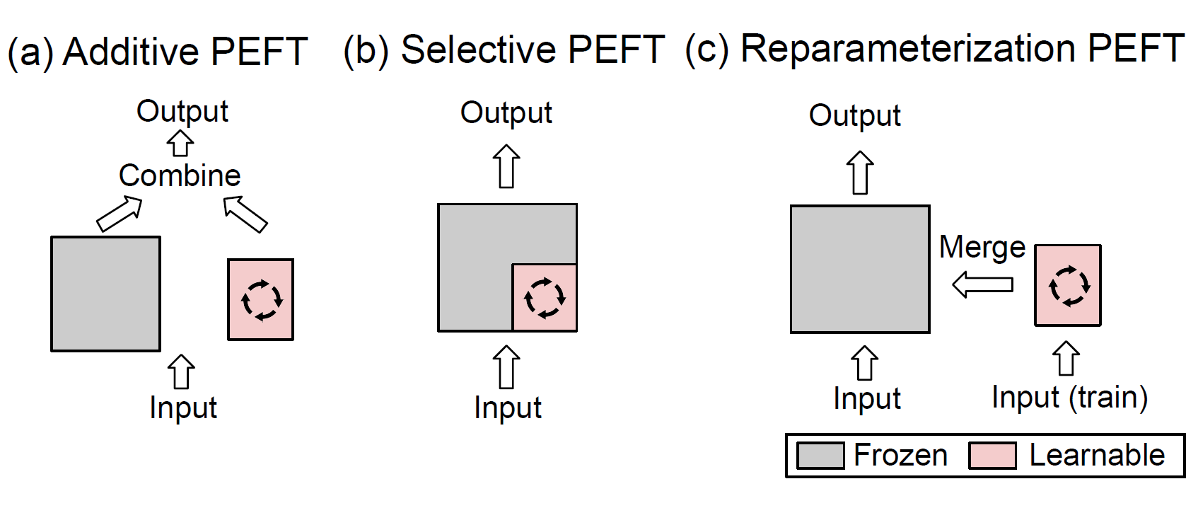
Figure 1: Comparison of FP8 and BF16 formats. Source: Smith et al. (2023)
Background
The topics of PFET are not that mathemaically complex, or … But understanding the minute details of LLMs is quite essential so i highly recommed reading the GPT2 architecture paper
Additive Finetuning
The basic idea in additive finetuning is to incorporate some more params into the LLM, Only these params are updated rest, the original params are kept frozen. So some obvious issuse with this approach is that it adds more params to an already large model, therby reducing infrence speeds.
Differnt methods propose differnt ways of implementing this, so the implementations can get a bit complicated.
Lest start with the simplest of Additive finetunign methods,
Prompt Tuning
Prompt tuning image from paper
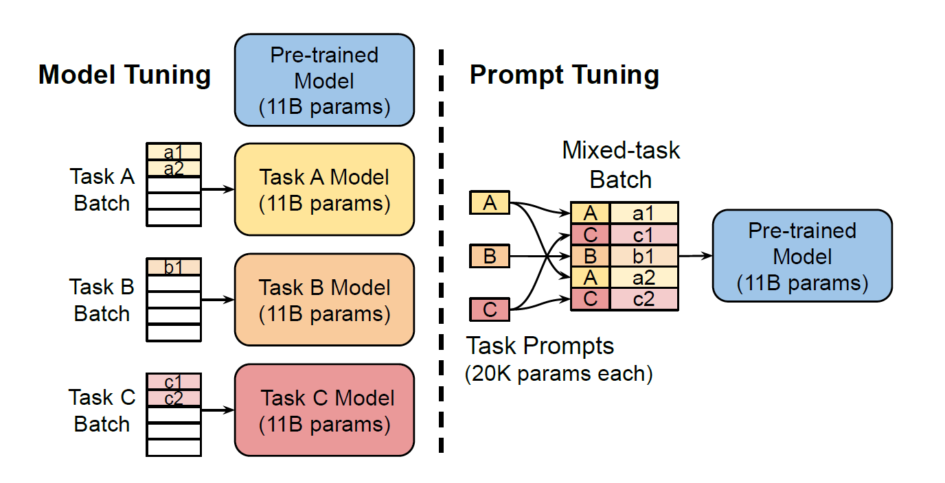
Figure 1: Comparison of FP8 and BF16 formats. Source: Smith et al. (2023)
Prompt tuning involves adding a few special embeddings, or “prompt vectors,” at the beginning of the input sequence. These vectors are not associated with any specific words in the model’s vocabulary; instead, they are learnable parameters designed to guide the model’s behavior for a particular task. For example, rather than manually crafting a prompt for sentiment analysis, the model learns optimal prompt vectors that maximize performance on the downstream task.
Mechanism of Prompt Tuning
- Initialization: The prompt vectors are randomly initialized and have the same dimensionality as the model’s word embeddings.
- Embedding Sequence: The input sequence for the model includes these special embeddings followed by the original input tokens.
- Training: During training, only the prompt vectors are updated, while the rest of the pre-trained model remains unchanged. This minimizes the number of parameters that need to be fine-tuned, making the process computationally efficient.
- Inference: For inference, the learned prompt vectors are prepended to the input sequence, allowing the model to perform the task effectively.
Advantages of Prompt Tuning
- Parameter Efficiency: Only a small number of parameters (the prompt vectors) need to be updated, drastically reducing storage requirements and making it easier to share models. Instead of sharing an entire 11-billion-parameter model, one can share just a few prompt vectors.
- Batch Processing: Prompt tuning enables the same base model to handle multiple tasks simultaneously. By including task-specific prompt vectors in the input, a single batch can contain examples from different tasks, streamlining the processing and improving efficiency.
Prompt-Tunig vs Fine Tuing vs Prompting
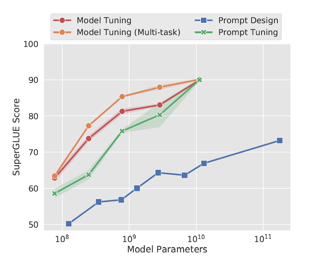
The blue line represents prompting, where natural language prompts are used without further training. The red and orange lines depict model fine-tuning, where the entire model is fine-tuned on downstream datasets, yielding the highest performance. The green line indicates prompt tuning.
Key Observations
- Smaller Models: Prompt tuning underperforms compared to full fine-tuning for smaller models. However, it still provides a significant improvement over plain prompting.
- Larger Models: The performance gap between prompt tuning and full model fine-tuning diminishes as model size increases. With large models, prompt tuning achieves comparable results to full fine-tuning, making it an efficient alternative.
Figure 1: Comparison of FP8 and BF16 formats. Source: Smith et al. (2023)
Prefix tuning
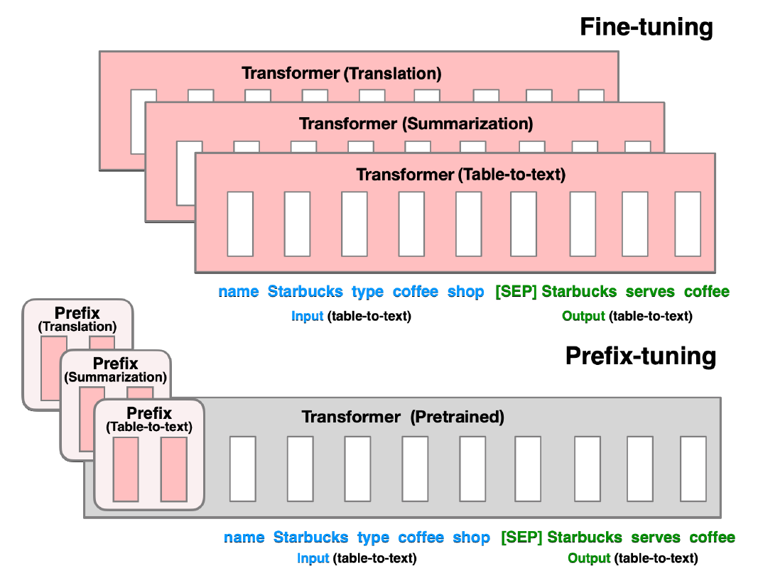
Figure 1: Comparison of FP8 and BF16 formats. Source: Smith et al. (2023)
Prefix tuning is similar to prompt tuning, but instead of appending prompt tokens only at the embedding layer, prefix tokens are added at every layer of the model.
Lets look at this in a bit more detail
In a standard Transformer architecture, each layer consists of two main components:
- Self-Attention Mechanism
- Feed-Forward Neural Network (FFN)
Prefix Tuning modifies this architecture by inserting prefixes before the self-attention layers of each Transformer block. Here’s how it works:
- Addition of Prefix Embeddings:
- Before Self-Attention: For each Transformer layer, a set of prefix embeddings (continuous vectors) is prepended to the input sequence. If the original input to a layer is represented as
x, the modified input becomes[PREFIX; x]. - Not Applied to FFN Layers: The prefixes are only added before the self-attention mechanisms, leaving the feed-forward layers unchanged.
- Impact on Self-Attention:
- Extended Input Sequence: By prepending prefixes, the self-attention mechanism now processes both the original tokens and the prefix tokens simultaneously.
- Attention Computation: The self-attention layers compute attention scores across the combined sequence (
[PREFIX; x]). This means that every token in the original input can attend to the prefix tokens and vice versa. - Guiding the Model: The prefix embeddings act as a continuous, task-specific context that influences how the model attends to and processes the input tokens. They effectively steer the model’s focus and generation behavior based on the learned prefixes.
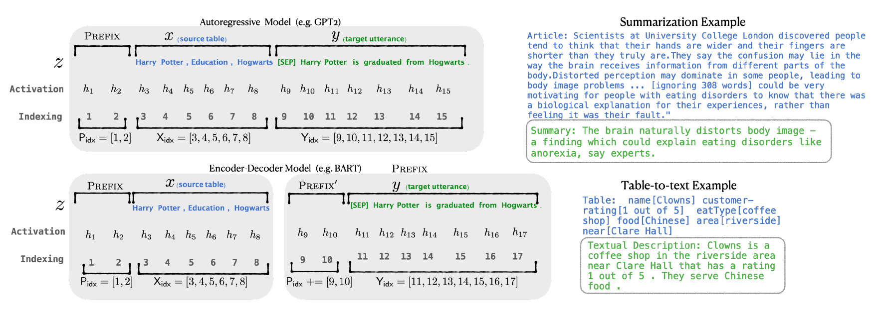
Figure 1: Comparison of FP8 and BF16 formats. Source: Smith et al. (2023)
adapters
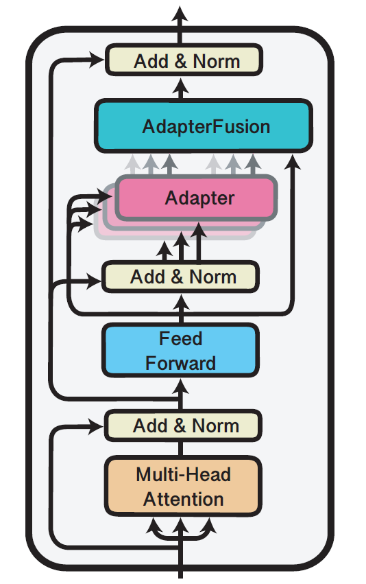
Figure 1: Comparison of FP8 and BF16 formats. Source: Smith et al. (2023)
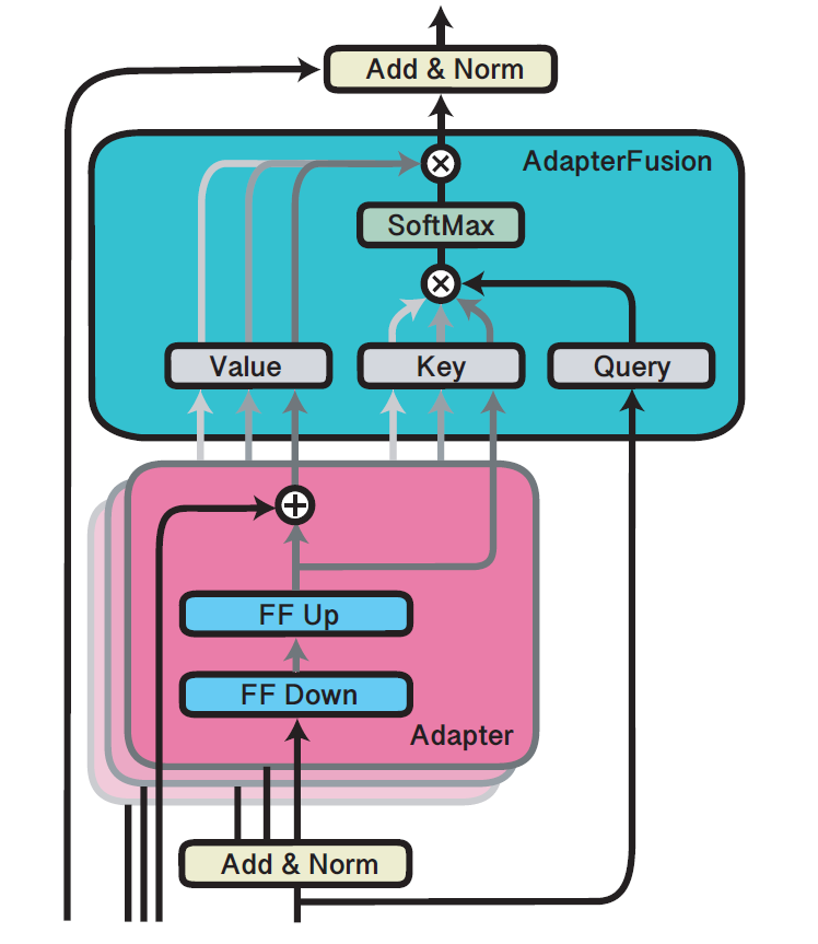
Figure 2: Comparison of FP8 and BF16 formats. Source: Smith et al. (2023)
adapter fusion
p-tuning
$(IA)^3$
Bitfit
lora
vera
dora
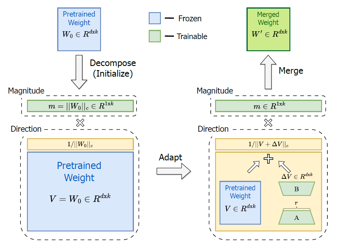
Figure 1: Comparison of FP8 and BF16 formats. Source: Smith et al. (2023)
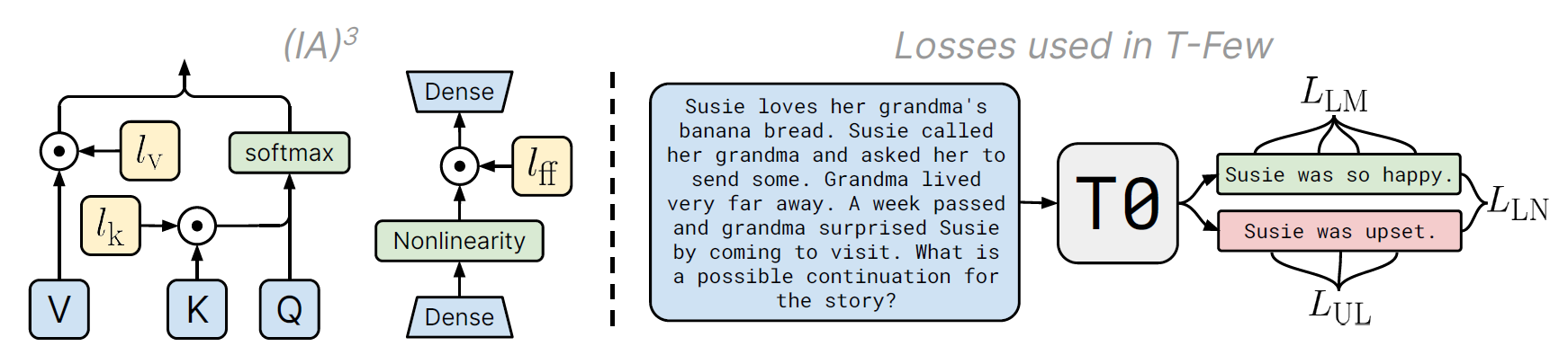
Figure 1: Comparison of FP8 and BF16 formats. Source: Smith et al. (2023)
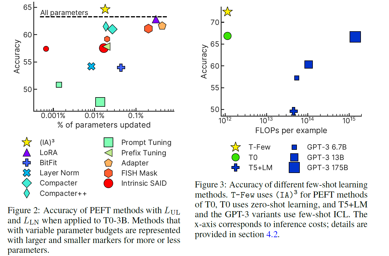
Figure 1: Comparison of FP8 and BF16 formats. Source: Smith et al. (2023)
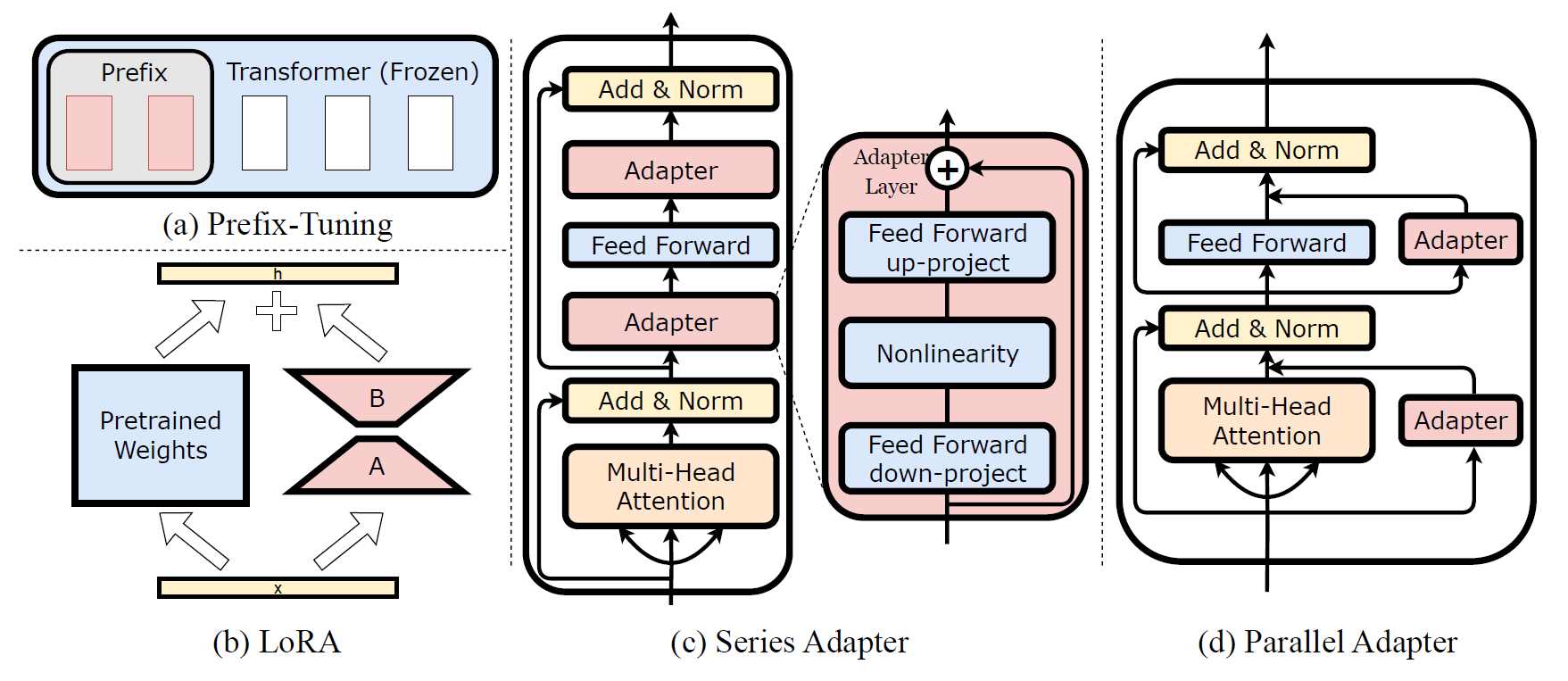
Figure 1: Comparison of FP8 and BF16 formats. Source: Smith et al. (2023)
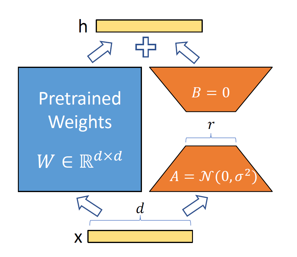
Figure 1: Comparison of FP8 and BF16 formats. Source: Smith et al. (2023)
Figure 1: Comparison of FP8 and BF16 formats. Source: Smith et al. (2023)
Figure 1: Comparison of FP8 and BF16 formats. Source: Smith et al. (2023)
Figure 1: Comparison of FP8 and BF16 formats. Source: Smith et al. (2023)
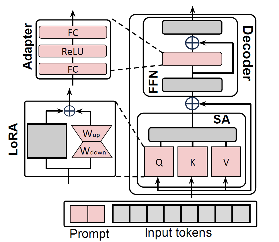
Figure 1: Comparison of FP8 and BF16 formats. Source: Smith et al. (2023)
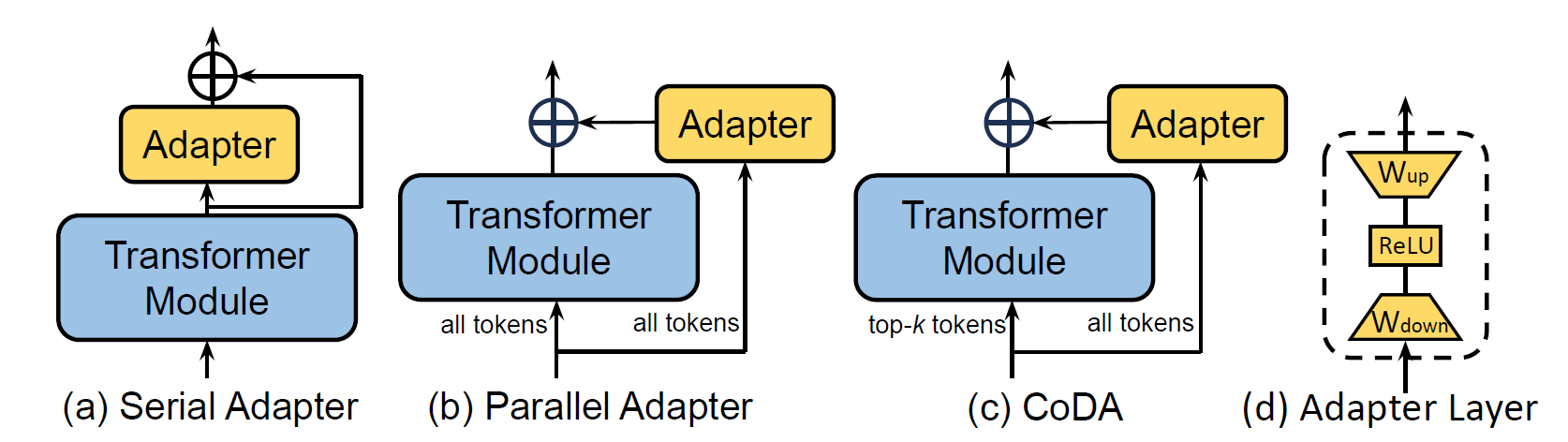
Figure 1: Comparison of FP8 and BF16 formats. Source: Smith et al. (2023)
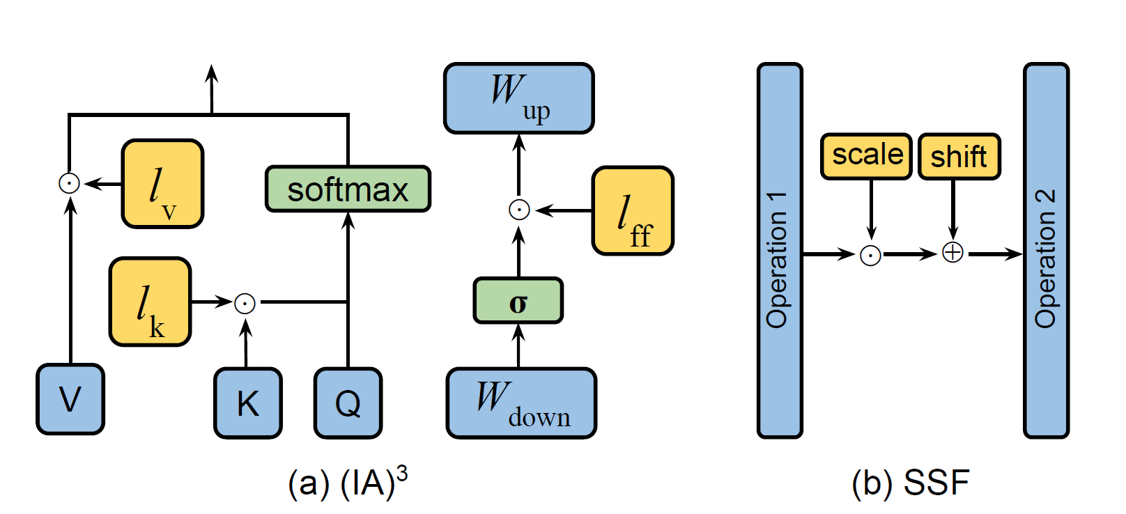
Figure 1: Comparison of FP8 and BF16 formats. Source: Smith et al. (2023)
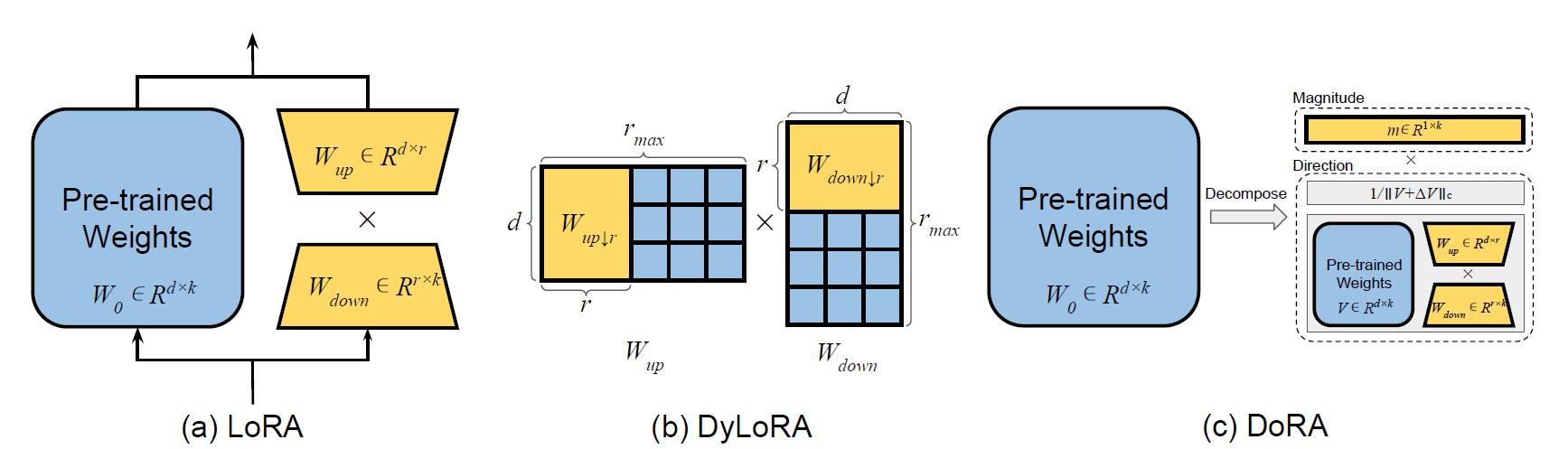
Figure 1: Comparison of FP8 and BF16 formats. Source: Smith et al. (2023)
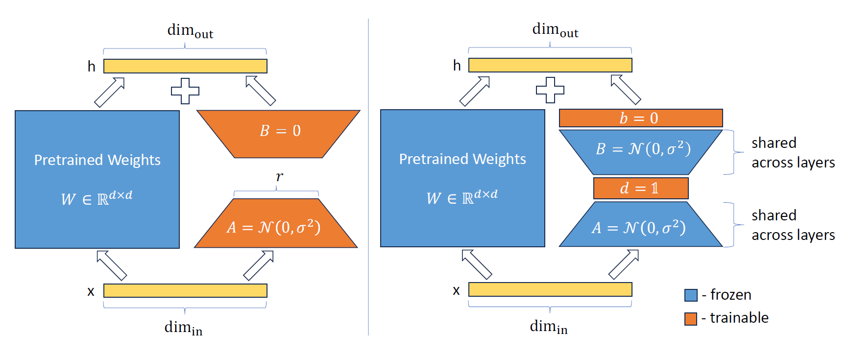
Figure 1: Comparison of FP8 and BF16 formats. Source: Smith et al. (2023)
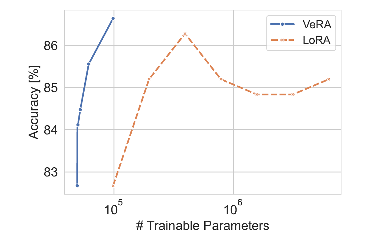
Figure 1: Comparison of FP8 and BF16 formats. Source: Smith et al. (2023)