ChatGPT can make mistakes. Check important info.
This disclaimer appears beneath the input field in ChatGPT and is not unique to it—similar notices can be found across all major large language models (LLMs). This is because one of the most well-known issues with LLMs is their tendency to hallucinate, meaning they can generate information that isn’t accurate or grounded in reality. So, before submitting your history paper directly from ChatGPT, make sure to proofread it carefully.
But why do LLMs hallucinate?
To understand this, consider how language models are trained. They learn through next-word prediction, effectively compressing vast amounts of training data to generate coherent text. However, given that the training data spans terabytes and the models themselves are only a few hundred gigabytes in size, some loss of information is inevitable. I like to think of hallucination as a form of information loss inherent to the model’s compression process.
Even when ChatGPT utilizes a web search tool like Bing to fetch answers, can we truly trust the information retrieved? 😅
Accuracy becomes crucial when dealing with more than just trivia. For instance, if you’re using a medical bot to diagnose symptoms or a legal bot to find relevant case law, precision is essential. This is where Retrieval Augmented Generation (RAG) comes into play. Although RAG has its own limitations, it provides a more reliable way to interact with LLMs by reducing the likelihood of hallucinations.
LLMs can also offer more confident answers when provided with the right context. However, retrieving relevant information is challenging, especially when dealing with millions of documents. LLMs have a limited context length, making it impossible to process all that data at once.
This is where Information Retrieval (IR) becomes essential—the unsung heroes in the race toward Artificial General Intelligence (AGI). By pairing a retriever with your language model, you establish the foundation of a RAG system. In this post, we’ll explore the retrieval aspect of RAG, and in the next installment, we’ll delve into the complete RAG pipeline.
Information Retrieval
The field of information retrieval is well-established, with its own standards and terminology. The information retrieval problem has been around as long as the internet itself, and while the solutions may not be as flashy as the latest LLM-based approaches, they effectively get the job done. Here, I’d like to highlight the two main methods for retrieving relevant documents:
- Sparse Retrieval
- Dense Retrieval
Let’s first examine sparse retrieval.
Sparse retrieval works on the BoW (Bag of Words) model, where the documents are indexed and an exact match in the query is used to retrieve the relevant document. The words in your query have to exactly match the words in the document present.
Let’s look at the inner workings of sparse retrieval starting with…
Term Document Matrix
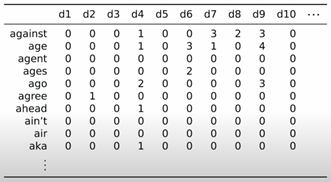
A term-document matrix (TDM) is a foundational tool in information retrieval and natural language processing. Each row in the matrix represents a word (term), and each column represents a document. The cells in this matrix record how many times each word appears in each document.
These matrices are typically very large and sparse. Despite this sparsity, term-document matrices hold significant latent information about the relationships between terms and documents, making them incredibly useful for identifying relevant documents based on specific query terms.
In actual practice, an inverted index is used. You can compare it to the adjacency matrix and adjacency list representations in graphs, where they are conceptually the same but more efficient to store in a linked list format. An inverted index is similar in many respects.
The basic approach is called TF-IDF (which stands for Term Frequency-Inverse Document Frequency).
TF-IDF Approach
TF-IDF is a common method for refining term-document values to extract more information about the relevance of documents. Here’s how TF-IDF works: # dont like this intro here, tells nothing about what tf-idf does just says “common method for refining term-document values to extract more information…” thats very bad
We start with a corpus of documents ($D$).
Term Frequency (TF):
- Term frequency is internal to each document. The TF of a word within a document is the number of times that word appears in the document divided by the total number of words in that document.
- Formula: $$ \text{TF}(w, \text{doc}) = \frac{\text{count}(w, \text{doc})}{|\text{doc}|} $$
Document Frequency (DF):
- Document frequency is a function of words and the entire corpus. It counts the number of documents that contain the target word, regardless of how often the word appears in each document.
- Formula: $$ \text{df}(w, D) = |\lbrace \text{doc} \in D : w \in \text{doc} \rbrace| $$
Inverse Document Frequency (IDF):
- Inverse document frequency is the log of the total number of documents divided by the document frequency.
- Formula: $$ \text{IDF}(w, D) = \log_e \left( \frac{|D|}{\text{df}(w, D)} \right) $$
TF-IDF Calculation:
- TF-IDF is the product of the TF and IDF values.
- Formula: $$ \text{TF-IDF}(w, \text{doc}, D) = \text{TF}(w, \text{doc}) \cdot \text{IDF}(w, D) $$
Understanding TF-IDF Values
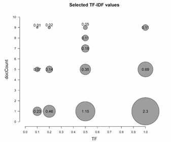
The image above shows TF-IDF values for various terms, highlighting the relationship between term frequency (TF) and document count (docCount).
TF-IDF values are highest for terms that appear frequently in a few documents. For instance, the largest bubble corresponds to a term with a high term frequency (TF close to 1.0) but appearing in only one document. This indicates that the term is highly specific to that document, making it a strong distinguishing feature.
Conversely, TF-IDF values are lowest for terms that appear infrequently across many documents. These terms are less helpful in distinguishing one document from another because their widespread presence dilutes their significance. For example, technical terms like “specificity” or “granularity” might appear in many documents but with low frequency in each, resulting in low TF-IDF values.
Retrieval Based on a Query
Relevance scores determine how well a document matches a user’s query. To calculate relevance scores for a query containing multiple terms, the standard approach is to sum the weights used in the term-document matrix. A common weighting scheme is TF-IDF (Term Frequency-Inverse Document Frequency).
The relevance score for a query $q$ in a document $\text{doc}$ within a corpus $D$ is:
$$ \text{RelevanceScore}(q, \text{doc}, D) = \sum_{w \in q} \text{TF-IDF}(w, \text{doc}, D) $$
Side Note:
Anybody who has dealt with the graph data structure knows that we mostly never use an adjacency matrix when working with graphs; we use an adjacency list. In a similar way, we don’t actually use the term-document matrix during actual use in a production system. Instead, we use something called an inverted index, which you can think of as an equivalent to an adjacency list. I used the term-document matrix for better visualization and simpler explanations.
BM25
BM25 is an advanced weighting scheme that builds upon TF-IDF to provide more accurate relevance scores in information retrieval. It addresses some of the limitations of TF-IDF by incorporating term frequency saturation and document length normalization.
Smoothed IDF
The first component of BM25 is the smoothed Inverse Document Frequency (IDF). This adjusts the IDF calculation to avoid zero values and provide more stable results:
$$ \text{IDF}_{BM25}(w, D) = \log_e \left( 1 + \frac{|D| - \text{df}(w, D) + 0.5}{\text{df}(w, D) + 0.5} \right) $$
Scoring
BM25 modifies term frequency (TF) to account for term frequency saturation, ensuring that the impact of term frequency increases are logarithmic rather than linear. The scoring formula is:
$$ \text{Score}_{BM25}(w, \text{doc}) = \frac{\text{TF}(w, \text{doc}) \cdot (k + 1)}{\text{TF}(w, \text{doc}) + k \cdot \left( 1 - b + b \cdot \frac{|\text{doc}|}{\text{avgdoclen}} \right)} $$
Here, $k$ and $b$ are parameters that control term frequency saturation and document length normalization, respectively. Typical values are $k = 1.2$ and $b = 0.75$.
BM25 Weight
Finally, the BM25 weight is calculated by combining the adjusted IDF values with the scoring values:
Why Dense Vector Representations?
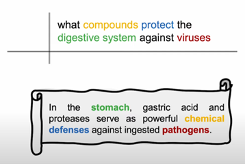
Sparse retrieval techniques, which rely on term matching, often fall short in understanding the semantic context of queries. For instance, a sparse approach might struggle to effectively link the query “what compounds protect the digestive system against viruses” with the relevant information that “gastric acid and proteases serve as powerful chemical defenses against ingested pathogens.” Dense vector representations, however, capture the deeper semantic meaning of words and phrases, enabling more accurate and context-aware retrieval of information. By transitioning to dense vectors, we can achieve significantly improved performance in understanding and responding to complex queries.
Before we move on to fancy dense retrieval techniques, I would like to make some points in favor of sparse retrieval.
- If your pretraining data doesn’t match the type of documents that you are trying to retrieve, then sparse retrieval techniques like BM25 will still work better.
- Generally, a mix of both sparse and dense retrieval is preferred. Sparse retrieval is used to fetch around 1,000 documents or sometimes more, and then dense retrieval techniques can be used to get the few documents necessary.
Neural Information Retrieval with Dense Vectors
In the realm of information retrieval (IR), the adoption of dense vector representations has significantly enhanced the efficiency and effectiveness of search systems. Traditional sparse retrieval techniques often fall short in capturing the nuanced semantic relationships between queries and documents. In contrast, dense vector representations, powered by neural networks, offer a richer, more expressive way to understand and match text.
Cross Encoders
Cross encoders are conceptually the simplest approach to neural IR. They work by concatenating the query and document texts into a single input, which is then processed through a pre-trained BERT model. The final output state above the [CLS] token is used for scoring.
Training and Loss Functions
Data and Encoding:
The dataset consists of triples $(q_i, \text{doc}_i^{+}, {\text{doc}_i^{-}})$, where $q_i$ is the query, $\text{doc}_i^{+}$ is a positive document, and ${\text{doc}_i^{-}}$ are negative documents.$$ \text{Rep}(q, \text{doc}) = \text{Dense}(\text{Enc}([q; \text{doc}])_{N, 0}) $$
Scoring:
The basis for scoring is the final output state above the [CLS] token, which is fed through a dense layer.Loss Function:
The loss function used for training is typically the negative log-likelihood of the positive passage:$$ \begin{align*} -\log \left( \frac{\exp(\text{Rep}(q_i, \text{doc}_i^{+}))} {\exp(\text{Rep}(q_i, \text{doc}_i^{+})) + \sum_{j=1}^n \exp(\text{Rep}(q_i, \text{doc}_i^{-}))} \right) \end{align*} $$
This loss function ensures that the model maximizes the score for the positive document while minimizing the scores for the negative documents, thereby refining the model’s ability to distinguish relevant documents from irrelevant ones.
While cross encoders are semantically rich due to the joint encoding of queries and documents, they are not scalable. This is because every document must be encoded at query time, which means that if we have a billion documents, we need to perform a billion forward passes with the BERT model for each query. This makes real-time retrieval infeasible.
Dense Passage Retriever (DPR)
DPR represents a scalable alternative by separately encoding queries and documents. Unlike cross encoders, DPR encodes queries and documents independently, allowing pre-encoding of documents, which enhances scalability.
Separate Encoding:
Queries and documents are encoded independently using a BERT-like model. The formula for the similarity score is:$$ \text{Sim}(q, \text{doc}) = \text{EncQ}(q)_{N,0}^T \text{EncD}(\text{doc})_{N,0} $$
- EncQ(q): The query $q$ is encoded into a dense vector representation using a BERT model.
- EncD(doc): The document $\text{doc}$ is similarly encoded into a dense vector.
Scoring:
The scoring function is the dot product of the query and document vectors, which efficiently measures their similarity.Loss Function:
The loss function for DPR is similar to that of cross encoders, but it uses the separately encoded vectors:$$ -\log \left( \frac{\exp(\text{Sim}(q_i, \text{doc}_i^{+}))}{\exp(\text{Sim}(q_i, \text{doc}_i^{+})) + \sum_{j=1}^n \exp(\text{Sim}(q_i, \text{doc}_i^{-}))} \right) $$
This loss function ensures that the positive document (i.e., the relevant document) is scored higher than the negative documents (i.e., irrelevant documents).
DPR is highly scalable as documents can be encoded offline. At query time, we only need to encode the query and compute the dot product with pre-encoded document vectors. This allows for efficient real-time retrieval. However, this approach loses the rich token-level interactions present in cross encoders, potentially reducing the expressivity of the model. The independent encoding may not capture the intricate relationships between query terms and document terms as effectively as the joint encoding in cross encoders.
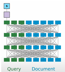
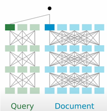
ColBERT
ColBERT (Contextualized Late Interaction over BERT) balances scalability and expressiveness by retaining some token-level interactions while ensuring efficiency. Here’s how ColBERT works:
Encoding:
Queries and documents are encoded using a BERT model. The encoding produces dense vector representations for each token in the query and the document.Scoring:
The scoring in ColBERT is based on a matrix of similarity scores between query tokens and document tokens. This matrix is computed by taking the dot product of each query token vector with each document token vector.$$ \text{MaxSim}(q, \text{doc}) = \sum_{i=1}^L \max_j \text{EncQ}(q)_{N,i}^T \text{EncD}(\text{doc})_{N,j} $$
Here’s a breakdown of this formula:
- EncQ(q) and EncD(doc): These represent the token-level embeddings for the query and document, respectively, produced by the BERT encoder.
- MaxSim: For each query token, we find the maximum similarity score across all document tokens, then sum these maximum values to get the overall similarity score.
Loss Function:
The loss function used for training is the negative log-likelihood of the positive passage, with MaxSim as the basis.$$ -\log \left( \frac{\exp(\text{MaxSim}(q_i, \text{doc}_i^{+}))}{\exp(\text{MaxSim}(q_i, \text{doc}_i^{+})) + \sum_{j=1}^n \exp(\text{MaxSim}(q_i, \text{doc}_i^{-}))} \right) $$
This loss function ensures that the model prioritizes the positive document by assigning it a higher score compared to negative documents.
ColBERT is highly scalable because documents can be pre-encoded and stored, requiring only the query encoding at runtime. This enables fast retrieval through efficient dot product calculations. Additionally, ColBERT retains semantic richness by allowing token-level interactions at the output stage, making it a powerful compromise between expressiveness and efficiency.
SPLADE
SPLADE (Sparse Latent Attributed Decoding Engine) introduces a novel approach by scoring with respect to the entire vocabulary rather than directly between query and document pairs. Here’s how SPLADE works:
Let’s break down this formula in detail:
SPLADE($t, w_j$): This represents the score for each vocabulary item $w_j$ given a token $t$.
$S_{ij}$: This score reflects the interaction between the $i$-th token in the sequence and the $j$-th vocabulary item. It is obtained by applying a transformation function to the inner product of the token embedding and the vocabulary embedding, plus a bias term $b_j$.
ReLU: The Rectified Linear Unit (ReLU) activation function is used to ensure that the scores are non-negative. This step helps in capturing only the significant interactions by zeroing out the negative values.
$\log(1 + \text{ReLU}(S_{ij}))$: Taking the logarithm of $1 + \text{ReLU}(S_{ij})$ smooths the scores and prevents very high values from dominating the overall score. This helps in achieving a more balanced distribution of scores.
Summation over $i$: The sum of the log-transformed scores across all tokens $i$ in the sequence aggregates their contributions to the score for the specific vocabulary item $w_j$. This results in a final SPLADE vector that is sparse, retaining only the most significant scores and thus reducing dimensionality and computational load.
Scoring:
The similarity function for SPLADE is the dot product of the sparse vectors for the query and document.$$ \text{Sim}_{\text{SPLADE}}(q, \text{doc}) = \text{SPLADE}(q)^T \text{SPLADE}(\text{doc}) $$
This scoring method ensures that the comparison is made across all vocabulary items, leveraging the sparsity of the vectors for efficiency.
Loss Function:
SPLADE includes a regularization term in its loss function to ensure sparsity and balanced scores.$$ \text{Loss} = -\log \left( \frac{\exp(\text{Sim}_{\text{SPLADE}}(q_i, \text{doc}_i^{+}))}{\exp(\text{Sim}_{\text{SPLADE}}(q_i, \text{doc}_i^{+})) + \sum_{j=1}^n \exp(\text{Sim}_{\text{SPLADE}}(q_i, \text{doc}_i^{-}))} \right) + \text{Reg} $$
The regularization term helps in maintaining the sparsity of the vectors, which is crucial for the efficiency of SPLADE.
SPLADE is efficient due to its use of sparse vectors, which reduces the computational overhead. By comparing sequences against the entire vocabulary, SPLADE captures a wide range of semantic information, making it versatile and effective in various retrieval scenarios. The regularization term ensures that the model produces balanced and sparse scores, optimizing both performance and computational efficiency.