A quick refresher on Autoregressive text generation
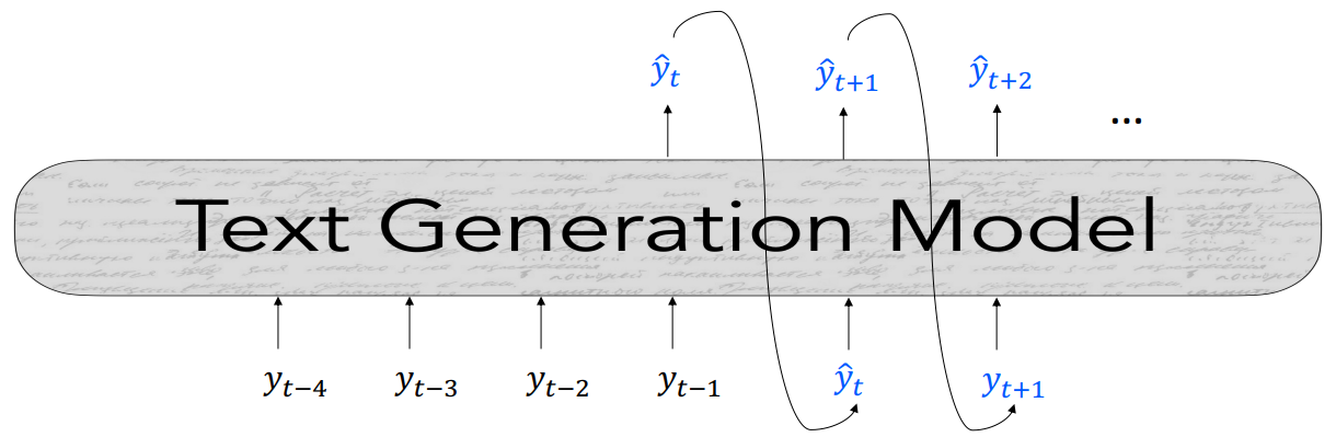
Autoregressive language models generate text through a sequential process of predicting one token at a time. The model takes a sequence of tokens $ \lbrace y \rbrace _{<t} $ as input and outputs a new token $ \hat{y_t} $. This process repeats iteratively, with each newly generated token becoming part of the input for the subsequent prediction.
At each time step $ t $, the model computes a vector of scores $ \mathbf{S} \in \mathbb{R}^V $, where $ V $ is the size of the vocabulary. For instance, in GPT-2, the vocabulary consists of 50,257 tokens.
$$ S = f(\lbrace y \rbrace _{<t} ) $$
The model then applies the softmax function to these scores to obtain a probability distribution over the vocabulary, representing the likelihood of each token being the next word given the preceding context.
$$ P(y_t = w \mid { y_{<t} }) = \frac{\exp(S_w)}{\sum_{w’ \in V} \exp(S_{w’})} $$
Here, $ S_w $ is the score of token $ w $, and the denominator is the sum of the exponentiated scores of all tokens in the vocabulary. Once we have this probability distribution, we can start decoding.
In the upcoming sections, we will explore different decoding methods, starting with greedy decoding, to understand how models convert these probabilities into coherent text.
Greedy Decoding
Greedy decoding is the most straightforward approach. Much like other classification tasks, where we take the argmax as the output, greedy decoding selects the token with the highest probability at each time step.
$$ \hat{y_t} = \arg\max_{w \in V} P(y_t = w \mid \lbrace y \rbrace _{<t}) $$
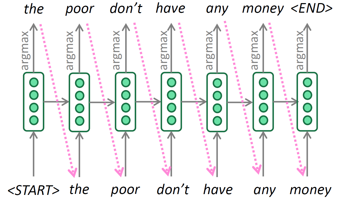
Below is an example of unconditional text generation. The model starts with a special <START> token, which can also be something like a newline character ‘\n’, and iteratively selects the most probable token at each step until it reaches the <END> token or some external maximum sequence length is met.
The issue with greedy decoding is that once a decision is made you can’t go back and change the decision, like there might have been a word like “a” or “the” If we could have taken it differently, we could eventually end up with a higher probability statement overall.
There is a simple way to get around this limitation of only considering one possible hypothesis.
Beam Search
The fundamental idea of beam search is to explore multiple hypotheses simultaneously rather than focusing on a single one. It keeps track of the $ k $ most probable partial sequences at each decoder step instead of just the top one. $ k $ is a parameter known as the beam width. This approach allows the algorithm to explore multiple hypotheses simultaneously, which improves the likelihood of finding a globally optimal sequence.
Beam Search Algorithm
- Starting Beam:
At time step $ t = 0 $, we start with the beam containing only the start-of-sequence token, denoted as $ \langle s \rangle $. Each sequence in the beam is paired with its cumulative log probability.
$$ \text{Beam}_0 = \lbrace{ \left( \langle s \rangle, \log P(\langle s \rangle) \right) }\rbrace $$
Since $ \langle s \rangle $ is the starting token, we often initialize its log probability to zero:
$$ \text{Beam}_0 = \lbrace{ \left( \langle s \rangle, 0 \right) } \rbrace $$
Expanding Sequences:
For each sequence $ Y_{1:t-1} $ in the beam, we generate all possible extensions by appending each possible next token $ \hat{y_t} $. Each extension forms a new candidate sequence:
$$ Y_{1:t} = Y_{1:t-1} \oplus \hat{y_t} $$
Here, $ \oplus $ denotes the concatenation of the existing sequence with the new token.
Computing Log Probabilities:
For each new candidate sequence $ Y_{1:t} $, we calculate the cumulative log probability. The log probability is used instead of the actual probability to prevent numerical underflow and to turn the product of probabilities into a sum, which is computationally more stable.
$$ \log P(Y_{1:t}) = \log P(\hat{y_t} \mid Y_{1:t-1}) + \log P(Y_{1:t-1}) $$
This combines the log probability of the new token $ \hat{y_t} $ given the previous sequence $ Y_{1:t-1} $ with the cumulative log probability of the previous sequence.
Generating Candidates:
Collect all possible candidates formed by extending each sequence in the current beam with all possible next tokens:
$$ \text{Candidates} = \lbrace{ (Y_{1:t-1} \oplus \hat{y_t}, \log P(\hat{y_t} \mid Y_{1:t-1}) + \log P(Y_{1:t-1})) } \rbrace $$
Pruning:
From the set of all candidates, select the top $ k $ sequences based on their log probabilities to form the new beam:
$$ \text{Beam}_t = \text{top}_k(\text{Candidates}) $$
This step ensures that only the $ k $ most probable sequences are kept, and the rest are discarded.
Repeating:
Repeat steps 2-5 until a stopping condition is met (e.g., maximum length reached or end token generated).
Final Output: After the iteration stops, we select the sequence with the highest cumulative log probability from the final beam.
$$ Y^\ast = \arg\max_{Y \in \text{Beam}_T} \log P(Y) $$
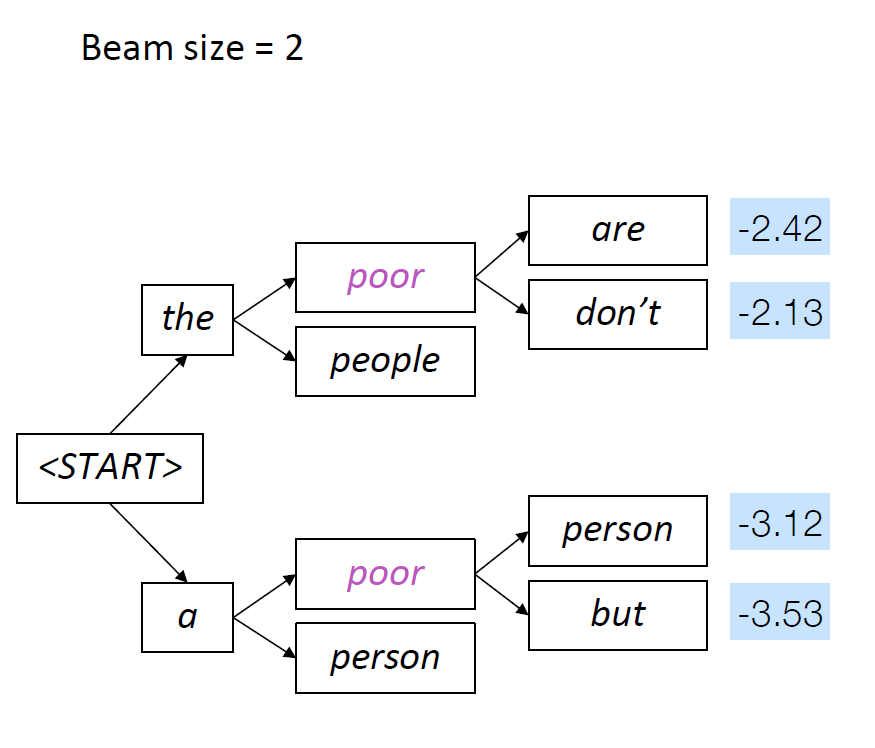
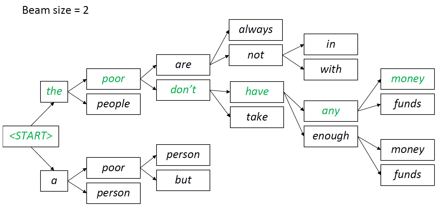
Beam Search with an Example of K =2
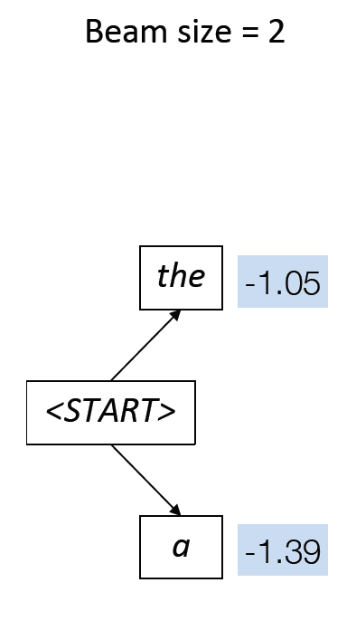
Get the two most probable tokens, rest are pruned.
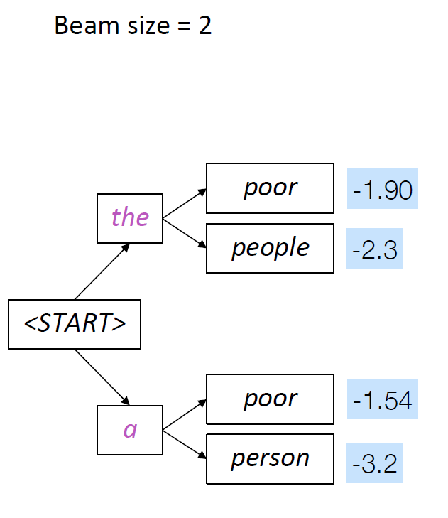
top 2 generations are “the poor” and “a poor”, these are kept and the reset are pruned
The above process is continued till we reach the <EOS> end of sequence token or reach a limit for max output tokens.
Greedy decoding and Beam Seach are some of the most popular approaches for decoding in LLM’s like chat GPT, Llama and Gemini.
The issue with these approaches.
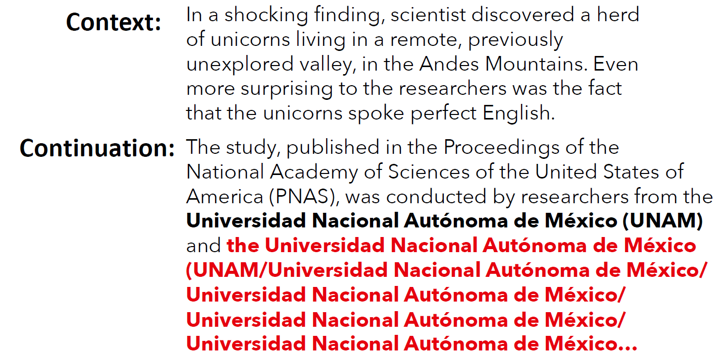
Even with substantial human context and the powerful GPT-2 Large language model, Beam Search (size 32) leads to degenerate repetition (highlighted in red). Source: Holtzman et al. (2020)
Open-ended text generation often leads to repetitive outputs. For example, when generating text about a unicorn trying to speak English, the continuation may initially appear coherent but soon start repeating phrases, like an institution’s name, excessively. This repetition happens because the language model assigns increasing probability to repeated sequences, as shown in the plot below of the model’s probability for the sequence “I don’t know.” Initially, the probability is regular, but as the phrase repeats, the probability increases, indicating the model is more confident about the repetition.
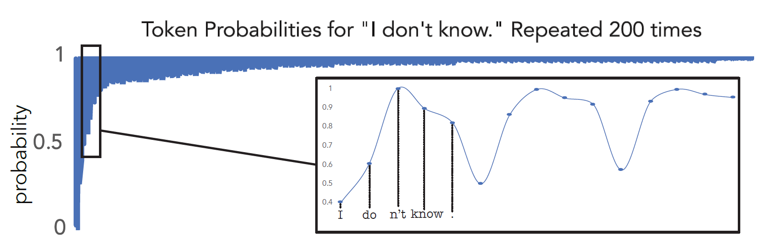
The probability of a repeated phrase increases with each repetition, creating a positive feedback loop. We found this effect to hold for the vast majority of phrases we tested, regardless of phrase length or if the phrases were sampled randomly rather than taken from human text. Source: Holtzman et al. (2020)
This issue, known as self-amplification, persists even with larger models. For instance, models with 175 billion parameters still suffer from repetition when generating the most likely string. Increasing scale alone does not resolve this problem. To mitigate repetition, one approach is n-gram blocking, which prevents the same n-gram from appearing twice. For example, if n is set to three, and the text contains “I am happy,” the next time “I am” appears, “happy” would be set to zero probability, preventing the repetition of this trigram. However, n-gram blocking has limitations, as it can eliminate necessary repetitions, such as a person’s name appearing multiple times.
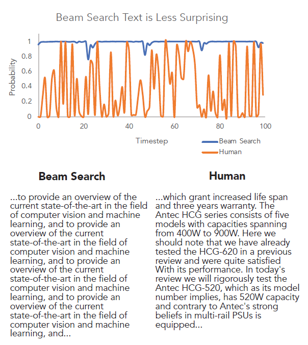
The probability assigned to tokens generated by Beam Search and humans, given the same context. Note the increased variance that characterizes human text, in contrast with the endless repetition of text decoded by Beam Search. Source: Holtzman et al. (2020)
Finally, let’s discuss whether generating the most likely string is reasonable for open-ended text generation. The answer is probably no, as it doesn’t align well with human patterns. In this graph, the orange curve represents human-generated text, while the blue curve shows machine-generated text using beam search. You can observe that human speech exhibits a lot of uncertainty, evident from the fluctuations in probabilities. For some words, humans are very certain, while for others, they are less sure. In contrast, the model distribution is always very confident, consistently assigning a probability of one to the sequence. This clear mismatch between the two distributions suggests that searching for the most likely string may not be the appropriate decoding objective.
Sampling Based Decoding
Another way of looking at the decoding problem is that we have a conditional probability distribution over the next token, why not just sample from this distribution?
Ancestral Sampling
At each time step, we’re going to draw a token from the probability distribution according to its relative likelihood. This process involves sampling a token from the distribution $ P(y_t = w \mid { y }_{<t}) $. Essentially, we are trying to sample $\hat{y_t}$ from this distribution.
Ancestral sampling allows us to select any token based on its probability, rather than being restricted to the most probable token.
$$ \hat{y_t} \sim P(y_t = w \mid { y }_{<t}) $$
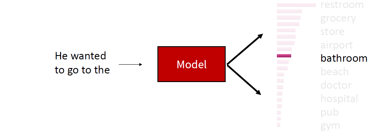
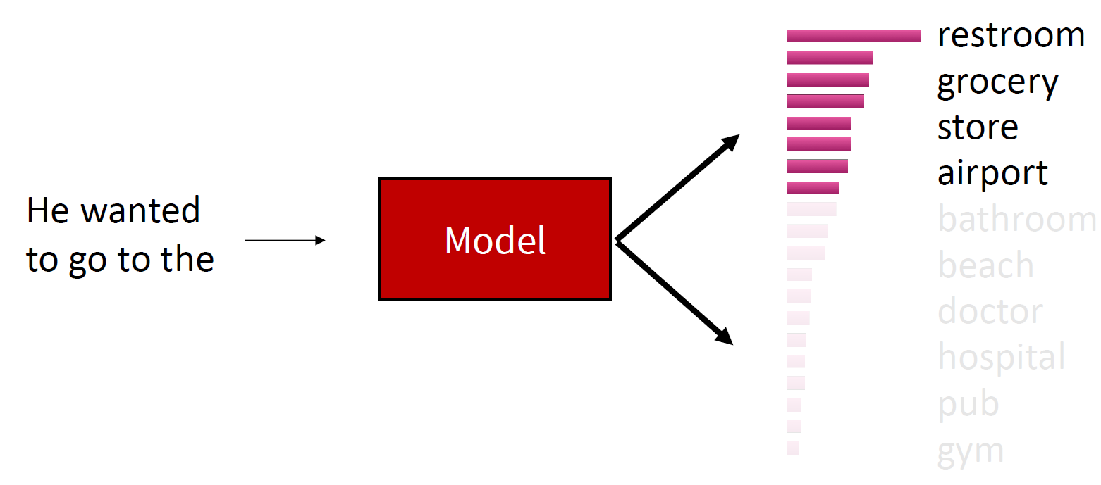
For example, previously you might have been restricted to selecting “restroom,” but with sampling, you might select “bathroom” as well.
Issues with ancestral sampling.
Sampling introduces a new set of challenges because it doesn’t completely eliminate the probabilities of any tokens. In vanilla sampling, every token in the vocabulary remains a potential option, which can sometimes result in generating inappropriate words. Even with a well-trained model, where most of the probability mass is concentrated on a limited set of suitable options, the distribution’s tail remains long due to the extensive vocabulary. This phenomenon, known as a heavy tail distribution, is characteristic of language. Consequently, when aggregated, the probabilities of these less likely tokens can still be significant.
For instance, many tokens may be contextually inappropriate, yet a good language model assigns each a very small probability. However, the sheer number of these tokens means that, collectively, they still have a considerable chance of being selected. To address this issue, we can cut off the tail by zeroing out the probabilities of the unwanted tokens.
Top $ k $ Sampling
One effective approach is top-$k$ sampling, where we only sample from the top $k$ tokens in the probability distribution. Increasing $k$ results in more diverse but potentially risky outputs, while decreasing $k$ leads to safer but more generic outputs.
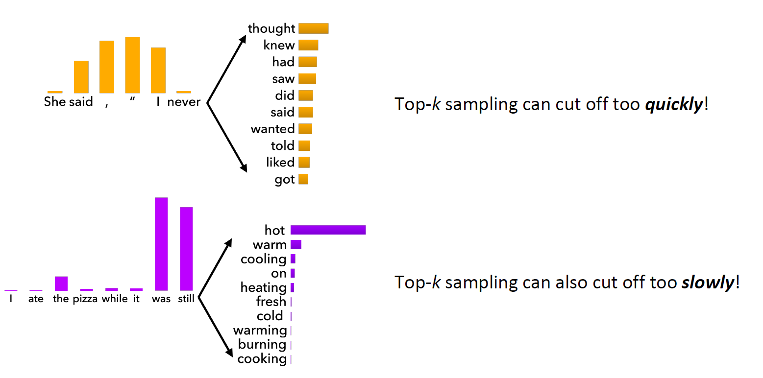
Top-$k$ decoding can present two major issues. First, it can cut off too quickly, as illustrated by the sentence “She said, ‘I never ___’.” Many valid options, such as “won’t” or “can’t,” might be excluded because they don’t fall within the top $k$ candidates, leading to poor recall for the generation system. Second, top-$k$ decoding can also cut off too slowly. For instance, in the sentence “ate the pizza while it was still ___,” the word “cold” is an unlikely choice according to common sense. Despite its low probability, the model might still sample “cold” as an output, resulting in poor precision for the generation model.
Given the problems with top-$k$ decoding, how can we address the issue that there is no single $k$ that fits all circumstances? The probability distributions we sample from are dynamic, and this variability causes issues. When the probability distribution is relatively flat, using a small $ k $ will eliminate many viable options, so we want $k$ to be larger in this case. Conversely, when the distribution is too peaky, a high $k$ would allow too many options to be viable. In this situation, we might want a smaller $k$ to be more selective.
Top $P$ sampling (nucleus sampling)
The solution might be that $k$ is just a suboptimal hyperparameter. Instead of focusing on $k$, we should consider sampling from tokens within the top $P$ probability percentiles of the cumulative distribution function (CDF). This approach adapts to the shape of the probability distribution and can provide a more flexible and effective sampling method.
The advantage of using top-$P$ sampling, where we sample from the top $P$ percentile of the cumulative probability mass, is that it effectively gives us an adaptive $k$ for each different probability distribution.
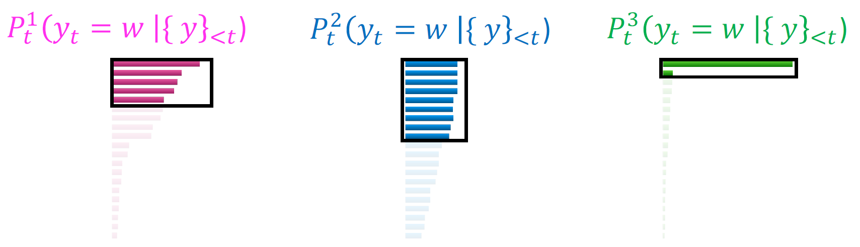
Let me explain what I mean by adaptive $k$. In the first distribution, which follows a typical power law of language, using top-$k$ sampling would mean selecting the top $k$ tokens. However, using top-$P$ sampling means we are focusing on the top $P$ percentile of the cumulative probability, which might be similar to top-K in this case.
For a relatively flat distribution like the blue one, top-$P$ sampling includes more candidates compared to top-$k$. On the other hand, for a more skewed distribution like the green one, top-$P$ sampling includes fewer candidates. By selecting the top $P$ percentile in the probability distribution, we achieve a more flexible $k$, which better reflects the good options in the model. This adaptive approach ensures that we are considering an appropriate number of candidates based on the shape of the distribution, leading to more effective sampling.
Epsilon Sampling
Epsilon sampling involves setting a threshold for lower bound probabilities. Essentially, if a word’s probability is less than a certain value, like 0.03, that word will never appear in the output distribution. This ensures that low-probability words are excluded from the final output.
Temperature Scaling
Another hyperparameter that we can tune to affect decoding is the temperature parameter $ \tau $. Recall that at each time step, the model computes a score for each word, and we use the softmax function to convert these scores into a probability distribution:
$$ P_t(y_t = w) = \frac{\exp(S_w)}{\sum_{w’ \in V} \exp(S_{w’})} $$
We can adjust these scores by introducing the temperature parameter $ \tau $. Specifically, we divide all scores $ S_w $ by $ \tau $ before applying the softmax function:
$$ P_t(y_t = w) = \frac{\exp(S_w / \tau)}{\sum_{w’ \in V} \exp(S_{w’} / \tau)} $$
This temperature adjustment affects the spread of the probability distribution without changing its monotonicity. For example, if word A had a higher probability than word B before the adjustment, it will still have a higher probability afterward, though the relative differences will change.
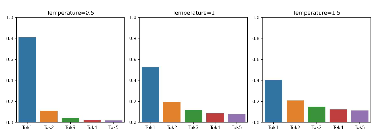
Raising the temperature $( \tau > 1 )$: The distribution $ P_t $ becomes more uniform (flatter). This means that the probabilities are more spread out across different words, leading to more diverse output.
Lowering the temperature $( \tau < 1 )$: The distribution $ P_t $ becomes more spiky. Probabilities are concentrated on the top words, resulting in less diverse output. In the extreme case, if $ \tau $ approaches zero, the probability distribution becomes a one-hot vector, concentrating all the probability mass on a single word, effectively reducing the method to argmax sampling (greedy decoding).
Temperature is a hyperparameter for decoding, similar to $ k $ in top-k sampling and $ P $ in top-p sampling. It can be tuned for both beam search and sampling algorithms and is orthogonal to the approaches we discussed before. Adjusting the temperature allows us to control the diversity of the generated output, balancing between exploring a wide range of options and focusing on the most likely ones.
Advanced decoding methods
So far, we’ve covered the basic ways language models generate text. But the world of natural language processing is always evolving, with new techniques popping up to make these models smarter and faster. In this section, we’ll explore some of these innovative decoding methods that are taking text generation to the next level.
Speculative Decoding
People don’t always need the latest and greatest large language models (LLMs) to solve their problems, especially since most of us spend our time asking simple questions like, “How many ‘r’s are in ‘strawberry’?” You don’t need OpenAI’s servers spinning up their massive trillion-parameter models for such straightforward queries when a much smaller model can provide the same answer. Using smaller models results in a lower memory footprint and more savings, which can also benefit the user. Therefore, why not use smaller models for simple questions and bring in the expert models when the smaller ones are not sufficient? This is a high-level overview of speculative decoding. Many prominent AI researchers believe that companies like OpenAI and Anthropic are implementing this approach when serving their models.
Understanding Speculative Decoding
Speculative decoding accelerates text generation by using a lightweight approximation model to generate multiple candidate tokens (called speculative tokens) in advance. These speculative tokens are then evaluated by the accurate but slower and larger target model. By accepting tokens that are probable under the target model and adjusting the distribution when the tokens produced by the approximation model do not align with the target model, we ensure that the final output matches what the target model would have produced—all without the time taken for sequential decoding from the larger models.
The key components of speculative decoding are:
- Target Model ($ M_p $): The accurate language model providing the true probability distribution $ p(x_t | x_{<t}) $.
- Approximation Model ($ M_q $): A faster, less accurate model approximating $ M_p $, providing $ q(x_t | x_{<t}) $.
- Prefix ($ x_{<t} $): The sequence of tokens generated so far.
- Completion Parameter ($ \gamma $): The number of speculative tokens generated.
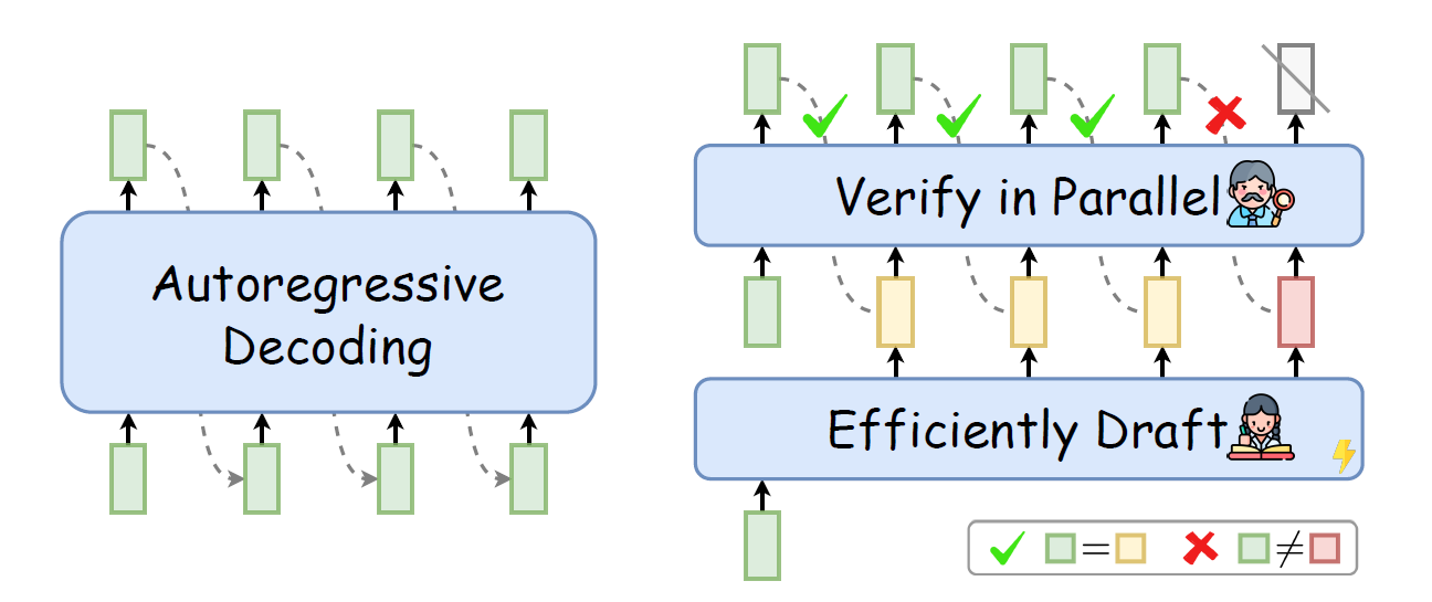
In contrast to autoregressive decoding (left) that generates sequentially, Speculative Decoding (right) first efficiently drafts multiple tokens and then verifies them in parallel using the target LLM. Drafted tokens after the bifurcation position (e.g., ) will be discarded to guarantee the generation quality. Source: Xia et al. (2020)
The Speculative Decoding Algorithm
The speculative decoding process combines outputs from both the approximation model and the target model to generate text more efficiently. It involves generating speculative tokens with the approximation model and then validating them with the target model. Here’s how it works:
Step 1: Generate Speculative Tokens with the Approximation Model
- Starting Point: Begin with the current prefix $ x_{<t} $.
- Speculative Generation: Use the approximation model $ M_q $ to generate $ \gamma $ speculative tokens $ x_1, x_2, \dots, x_\gamma $ in an autoregressive manner. Each token is generated based on the prefix and any previously generated speculative tokens.
Step 2: Evaluate Speculative Tokens with the Target Model
- Probability Computation: For each speculative token $ x_i $, compute the target model’s probability distribution $ p_i(x) $ based on the extended prefix up to $ x_i $.
- Purpose: This assesses how likely each speculative token is under the target model, allowing us to decide whether to accept it.
Step 3: Decide Whether to Accept Each Speculative Token
- Acceptance Probability: For each speculative token $ x_i $, calculate: $$ a_i = \min\left(1, \frac{p_i(x_i)}{q_i(x_i)}\right) $$
- Random Sampling: Generate a random number $ r_i $ between 0 and 1.
- Acceptance Criterion:
- Accept $ x_i $ if $ r_i \leq a_i $.
- Reject $ x_i $ if $ r_i > a_i $, and discard all subsequent speculative tokens (since they depend on the rejected token).
Step 4: Adjust the Probability Distribution if Needed
- When to Adjust: If a token is rejected.
- Adjusted Distribution: Compute the adjusted target model distribution for the next token: $$ p’(x) = \text{norm}\left(\max\left(0, p_{n+1}(x) - q_{n+1}(x)\right)\right) $$ where $ n $ is the number of accepted speculative tokens.
- Purpose: This adjustment accounts for the probability mass already covered by the accepted speculative tokens, ensuring correct sampling for the next token.
Step 5: Generate the Next Token from the Target Model
- Sampling: Draw the next token $ t $ from the adjusted distribution $ p’(x) $ using the target model $ M_p $.
- Update Prefix: Extend the current prefix by appending the accepted speculative tokens and the new token $ t $.
- Iterate: Repeat the process starting from Step 1 with the updated prefix.
Detailed Example
To illustrate the speculative decoding algorithm, let’s walk through a concrete example.
Assumptions:
- Target Model ($ M_p $): An accurate but slower language model.
- Approximation Model ($ M_q $): A faster, less accurate model.
- Prefix: “The quick brown”.
- Vocabulary: Includes words like “fox”, “dog”, “cat”, “jumps”, etc.
- Completion Parameter ($ \gamma $): Set to 2.
Step 1: Sampling Guesses from $ M_q $
Iteration 1 ($ i = 1 $)
We run $ M_q $ on the prefix “The quick brown” to compute $ q_1(x) $. Suppose $ q_1(\text{fox}) = 0.6 $, $ q_1(\text{dog}) = 0.3 $, and $ q_1(\text{cat}) = 0.1 $. We sample $ x_1 $ from $ q_1(x) $, and let’s say we get $ x_1 = \text{fox} $.
Iteration 2 ($ i = 2 $)
Next, we run $ M_q $ on the extended prefix “The quick brown fox” to compute $ q_2(x) $. Suppose $ q_2(\text{jumps}) = 0.5 $, $ q_2(\text{sleeps}) = 0.3 $, and $ q_2(\text{runs}) = 0.2 $. We sample $ x_2 $ from $ q_2(x) $, and let’s say we get $ x_2 = \text{jumps} $.
Step 2: Evaluating with $ M_p $
We compute the true probability distributions using $ M_p $:
- $ p_1(x) $ for the prefix “The quick brown”: Suppose $ p_1(\text{fox}) = 0.7 $, $ p_1(\text{dog}) = 0.2 $, $ p_1(\text{cat}) = 0.1 $.
- $ p_2(x) $ for the prefix “The quick brown fox”: Suppose $ p_2(\text{jumps}) = 0.6 $, $ p_2(\text{sleeps}) = 0.2 $, $ p_2(\text{runs}) = 0.2 $.
- $ p_3(x) $ for the prefix “The quick brown fox jumps”: Suppose $ p_3(\text{over}) = 0.8 $, $ p_3(\text{high}) = 0.1 $, $ p_3(\text{quickly}) = 0.1 $.
Step 3: Determining Acceptance
For $ x_1 = \text{fox} $:
We calculate the acceptance probability $ a_1 = \min\left(1, \frac{p_1(\text{fox})}{q_1(\text{fox})}\right) = \min\left(1, \frac{0.7}{0.6}\right) = 1 $. We generate a random number $ r_1 $, say $ r_1 = 0.5 $. Since $ r_1 \leq a_1 $, we accept $ x_1 = \text{fox} $.
For $ x_2 = \text{jumps} $:
We calculate $ a_2 = \min\left(1, \frac{p_2(\text{jumps})}{q_2(\text{jumps})}\right) = \min\left(1, \frac{0.6}{0.5}\right) = 1 $. We generate $ r_2 = 0.8 $. Since $ r_2 \leq a_2 $, we accept $ x_2 = \text{jumps} $.
We have accepted both speculative tokens, so $ n = 2 $.
Step 4: Adjusting the Distribution
Since we have accepted all speculative tokens, we adjust the distribution for the next token. We set $ p’(x) = p_3(x) $ and compute $ q_3(x) $ using $ M_q $ on the prefix “The quick brown fox jumps”. Suppose $ q_3(\text{over}) = 0.7 $, $ q_3(\text{high}) = 0.2 $, and $ q_3(\text{quickly}) = 0.1 $.
We adjust $ p’(x) $ by subtracting $ q_3(x) $ and normalizing:
- $ p’(\text{over}) = \max(0, 0.8 - 0.7) = 0.1 $
- $ p’(\text{high}) = \max(0, 0.1 - 0.2) = 0 $
- $ p’(\text{quickly}) = \max(0, 0.1 - 0.1) = 0 $
After normalization (since total mass is 0.1), we have $ p’(\text{over}) = 1.0 $.
Step 5: Generating the Next Token
We sample $ t $ from $ p’(x) $, which must be “over” since $ p’(\text{over}) = 1.0 $. We construct the new prefix by adding the accepted tokens and the new token: “The quick brown fox jumps over”.
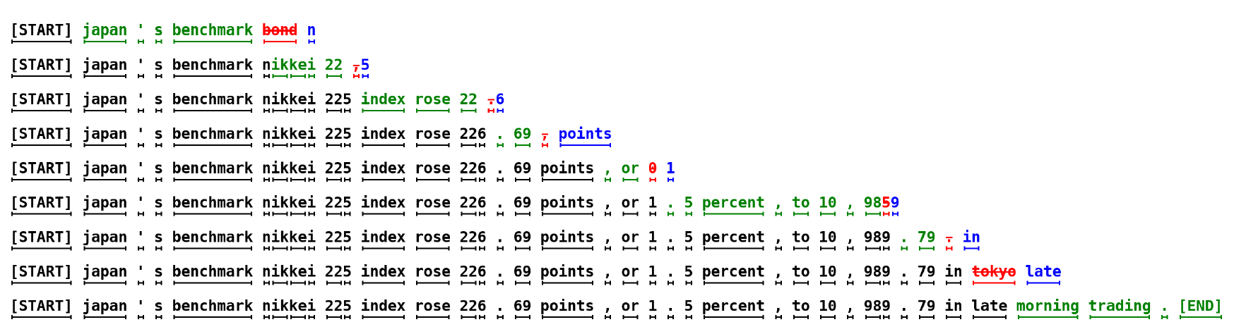
Each line represents one iteration of the algorithm. The green tokens are the suggestions made by the approximation model (here, a GPT-like Transformer decoder with 6M parameters trained on lm1b with 8k tokens) that the target model (here, a GPT-like Transformer decoder with 97M parameters in the same setting) accepted, while the red and blue tokens are the rejected suggestions and their corrections, respectively. For example, in the first line the target model was run only once, and 5 tokens were generated. Source: Leviathan et al. (2020)
Why Speculative Decoding Works
At first glance, speculative decoding might seem counterintuitive—using two models and computing probabilities twice to save time? I had the same skepticism when I first encountered the concept. How could this approach possibly be more efficient when it appears we’re doubling our efforts?
The key lies in understanding the autoregressive nature of language models. Traditionally, generating each token sequentially with a large model is time-consuming because each new token depends on all the previous ones, which prevents any form of parallel processing. This sequential dependency was a major bottleneck that frustrated many users, including myself, who experienced slower generation speeds with models like GPT-4.
Speculative decoding offers a clever workaround. By leveraging a lightweight approximation model, we can generate multiple speculative tokens in advance. Since this approximation model is both fast and efficient, producing these tokens doesn’t add much overhead. Imagine having a smaller, distilled version of the model doing the heavy lifting upfront—it feels almost like having an assistant that anticipates your next move.
Once these speculative tokens are generated, the more accurate but slower target model steps in to evaluate them. This evaluation happens in parallel, significantly reducing the overall latency compared to the traditional sequential approach. It’s like having the best expert in the room quickly vet a batch of suggestions from the assistant, ensuring that only the most probable and relevant tokens make it to the final output.
What truly makes speculative decoding work is this balance between speed and accuracy. By accepting tokens that align well with what the target model would produce, we maintain the quality of the output without the painstakingly slow generation process. It’s an elegant solution that not only speeds things up but also preserves the integrity of the responses, making the entire system more efficient and user-friendly.
Practical Considerations
Choosing the Completion Parameter ($ \gamma $)
There is a trade-off in selecting $ \gamma $. A larger $ \gamma $ increases the chance of accepting more tokens, potentially accelerating the decoding process, but it also adds computational overhead due to the increased number of computations required by $ M_p $ and $ M_q $. It’s important to balance $ \gamma $ based on model performance and available resources.
Quality of the Approximation Model
The effectiveness of speculative decoding depends on the approximation quality of $ M_q $. A closer match between $ q(x) $ and $ p(x) $ leads to higher acceptance rates, improving efficiency. However, $ M_q $ must be significantly faster than $ M_p $ to justify its use.
References:
[1] https://arxiv.org/pdf/1904.09751
[2] https://arxiv.org/pdf/2401.07851v3
[3] https://arxiv.org/pdf/2211.17192
[4] https://people.cs.umass.edu/~miyyer/cs685/